Nonlinear Systems of Equations: Fixed-Point Iteration Method

The Method

Similar to the fixed-point iteration method for finding roots of a single equation, the fixed-point iteration method can be extended to nonlinear systems. This is in fact a simple extension to the iterative methods used for solving systems of linear equations. The fixed-point iteration method proceeds by rearranging the nonlinear system such that the equations have the form.

where is a nonlinear function of the components . By assuming an initial guess, the new estimates can be obtained in a manner similar to either the Jacobi method or the Gauss-Seidel method described previously for linear systems of equations. Similar to linear systems of equations, the Euclidean norm can be used to check convergence. So, if the components of the vector after iteration are , and if after iteration the components are: , then, the stopping criterion would be:

where

Note that any other norm function can work as well.

Example

Use the fixed-point iteration method with to find the solution to the following nonlinear system of equations:

Solution

The exact solution in the field of real numbers for this system can actually be obtained using Mathematica as shown in the code below.

Clear[x1, x2];
a = Solve[{x1^2 + x1*x2 == 10, x2 + 3 x1*x2^2 == 57}, {x1, x2}, Reals]
N[a]

import sympy as sp
sp.init_printing(use_latex=True)
x1, x2 = sp.symbols('x1 x2')
a = sp.nonlinsolve([x1**2 + x1*x2 - 10, x2 + 3*x1*x2**2 - 57], [x1, x2])
display(a)

The fixed-point iteration numerical method requires rearranging the equations first to the form:

The following is a possible rearrangement:

Using an initial guess of and yields the following:

For the next iteration, we get:

Continuing the procedure shows that it is diverging. A different rearrangement for the equations has the form:

Using the same initial guesses, the first iteration produces:

The value of after the first iteration is:

The following Microsoft Excel table shows that convergence to and satisfying the required criterion is achieved after 9 iterations.

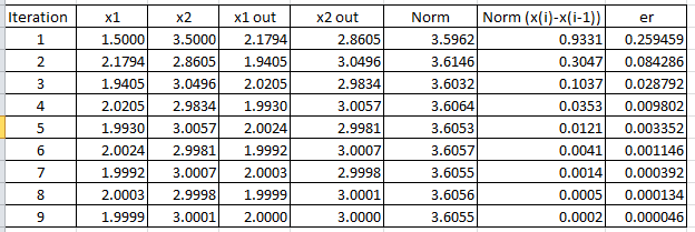
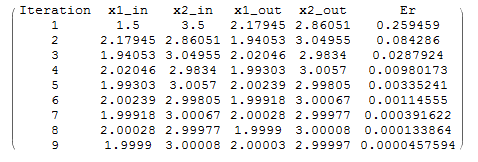
The following code does the same thing in Mathematica to produce the table below:

xtable = {{1.5, 3.5}};
ErrorTable = {1};
Nmax = 100;
eps = 0.0001;
i = 2;
While[And[ErrorTable[[i - 1]] > eps, i <= Nmax], 
  x1new = Sqrt[10 - xtable[[i - 1, 1]]*xtable[[i - 1, 2]]]; 
  x2new = Sqrt[(57 - xtable[[i - 1, 2]])/3/x1new]; 
  xnew = {x1new, x2new};
  xtable = Append[xtable, xnew]; 
  er = Norm[xnew - xtable[[i - 1]]]/Norm[xnew]; 
  ErrorTable = Append[ErrorTable, er]; i = i + 1];
Title = {"Iteration", "x1_in", "x2_in", "x1_out", "x2_out", "Er"};
T2 = Table[{i, xtable[[i, 1]], xtable[[i, 2]], xtable[[i + 1, 1]], xtable[[i + 1, 2]], ErrorTable[[i + 1]]}, {i, 1, Length[xtable] - 1}];
T2 = Prepend[T2, Title];
T2 // MatrixForm

import numpy as np
import pandas as pd
xtable = np.array([[1.5, 3.5]])
ErrorTable = [1]
Nmax = 100
eps = 0.0001
i = 1
while ErrorTable[i - 1] > eps and i <= Nmax: 
  x1new = np.sqrt(10 - xtable[i - 1, 0]*xtable[i - 1, 1]) 
  x2new = np.sqrt((57 - xtable[i - 1, 1])/3/x1new)
  xnew = [x1new, x2new]
  xtable = np.concatenate((xtable,[xnew])) 
  er = np.linalg.norm(xnew - xtable[i - 1])/np.linalg.norm(xnew) 
  ErrorTable.append(er)
  i += 1
T2 = [[i+1, xtable[i][0], xtable[i][1], xtable[i + 1][0], xtable[i + 1][1], ErrorTable[i + 1]] for i in range(len(xtable)-1)]
pd.DataFrame(T2, columns=["Iteration", "x1_in", "x2_in", "x1_out", "x2_out", "Er"])

MATLAB files for the fixed-point iteration example:
Download MATLAB file 1 (fpisystem.m)
Download MATLAB file 2 (g1.m)
Download MATLAB file 3 (g2.m)

The example here shows that the fixed-point iteration method is not guaranteed to give a possible solution. In fact, the initial guess and the form chosen affect whether a solution can be obtained or not. Note that the “FixedPointList” built-in function in Mathematica can be used to implement the method with an initial guess. Notice in the code below how the function outputs the vector as a list and that the second component uses the output of the first component:

g[x_] := (x1 = Sqrt[10 - x[[1]]*x[[2]]]; {x1, Sqrt[(57 - x[[2]])/3/x1]})
FixedPointList[g[#] &, {1.5, 3.5}, 20]

import numpy as np
def g(x):
  x1 = np.sqrt(10 - x[0]*x[1])
  return [x1, np.sqrt((57 - x[1])/3/x1)]
x = [1.5, 3.5]
for i in range(20):
  print(x)
  x = g(x)

Lecture Video