Engineering at Alberta Courses » Fixed-Point Iteration Method

Open Methods: Fixed-Point Iteration Method

The Method

Let $g:V\rightarrow V$ . A fixed point of $g$ is defined as $x\in V$ such that $x=g(x)$ . If $g:\mathbb{R}\rightarrow \mathbb{R}$ , then a fixed point of $g$ is the intersection of the graphs of the two functions $f(x)=x$ and $g(x)$ .

The fixed-point iteration method relies on replacing the expression $f(x)=0$ with the expression $x=g(x)$ . Then, an initial guess for the root $x_1$ is assumed and input as an argument for the function $g$ . The output $g(x_1)$ is then the estimate $x_2$ . The process is then iterated until the output $x_{n+1}\approx g(x_n)$ . The following is the algorithm for the fixed-point iteration method. Assuming $x_0$ , $\varepsilon_s$ , and maximum number of iterations $N$ :
Set $x_{n+1}=g(x_n)$ , and calculate $\varepsilon_r=\frac{x_{n+1}-x_{n}}{x_{n+1}}$ and compare with $\varepsilon_s$ . If $|\varepsilon_r|\leq \varepsilon_s$ or if $n=N$ , then stop the procedure, otherwise, repeat.

The Babylonian method for finding roots described in the introduction section is a prime example of the use of this method. If we seek to find the solution for the equation $x^2=s$ or $f(x)=x^2-s=0$ , then a fixed-point iteration scheme can be implemented by writing this equation in the form:

$x=\frac{x+\frac{s}{x}}{2}$

Example

Consider the function $f(x)=\cos{x}-x$ . We wish to find the root of the equation $f(x)=0$ , i.e., $\cos{x}-x=0$ . The expression can be rearranged to the fixed-point iteration form $x=\cos{x}$ and an initial guess $x_0=0.1$ can be used. The tolerance $\varepsilon_s$ is set to 0.001. The following is the Microsoft Excel table showing that the tolerance is achieved after 19 iterations:
excel1

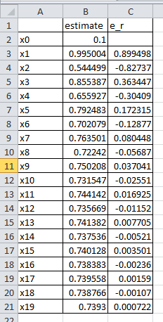
Mathematica has a built-in algorithm for the fixed-point iteration method. The function “FixedPoint[f,Expr,n]” applies the fixed-point iteration method $x=f(x)$ with the initial guess being “Expr” with a maximum number of iterations “n”. As well, the function “FixedPointList[f,Expr,n]” returns the list of applying the function “n” times. If “n” is omitted, then the software applies the fixed-point iteration method until convergence is achieved. Here is a snapshot of the code and the output for the fixed-point iteration $x=\cos{x}$ . The software finds the solution $x=0.739085$ . Compare the list below with the Microsoft Excel sheet above.
fixedpoint1

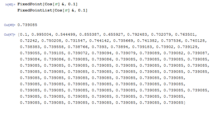
Alternatively, simple code can be written in Mathematica with the following output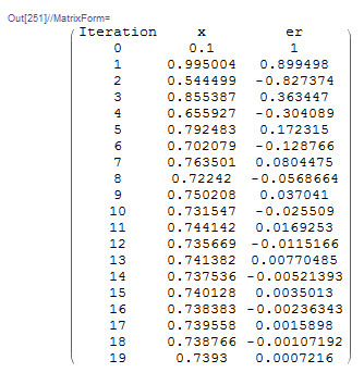
fixedpoint2

View Mathematica Code

x = {0.1};
er = {1};
es = 0.001;
MaxIter = 100;
i = 1;
While[And[i <= MaxIter, Abs[er[[i]]] > es],  xnew = Cos[x[[i]]]; x = Append[x, xnew]; ernew = (xnew - x[[i]])/xnew; er = Append[er, ernew]; i++];
T = Length[x];
SolutionTable = Table[{i - 1, x[[i]], er[[i]]}, {i, 1, T}];
SolutionTable1 = {"Iteration", "x", "er"};
T = Prepend[SolutionTable, SolutionTable1];
T // MatrixForm

View Python Code

import numpy as np
import pandas as pd

x = [0.1]
er = [1]
es = 0.001
MaxIter = 100
i = 0
while i <= MaxIter and abs(er[i]) > es:
  xnew = np.cos(x[i])
  x.append(xnew)
  ernew = (xnew - x[i])/xnew
  er.append(ernew)
  i+=1
SolutionTable = [[i, x[i], er[i]] for i in range(len(x))]
pd.DataFrame(SolutionTable, columns=["Iteration", "x", "er"])

The following MATLAB code runs the fixed-point iteration method to find the root of a function $f(x)$ with initial guess $x_0$ . The value of the estimate and approximate relative error at each iteration is displayed in the command window. Additionally, two plots are produced to visualize how the iterations and the errors progress. Your function should be written in the form $x = g(x)$ . Then call the fixed point iteration function with fixedpointfun2(@(x) g(x), x0). For example, try fixedpointfun2(@(x) cos(x), 0.1)

MATLAB file Download

Convergence

The fixed-point iteration method converges easily if in the region of interest we have $|g'(x)|<1$ . Otherwise, it does not converge. Here is an example where the fixed-point iteration method fails to converge.

Example

Consider the function $f(x)=\sin{5x}+\cos{2x}$ . To find the root of the equation $f(x)=0$ , the expression can be converted into the fixed-point iteration form as:
$x=\sin{5x}+\cos{2x}+x$ . Implementing the fixed-point iteration procedure shows that this expression almost never converges but oscillates:

View Mathematica Code

Clear[x, g]
x = {-0.9};
er = {1};
es = 0.001;
MaxIter = 100;
i = 1;
g[x_] := (Sin[5 x] + Cos[2 x]) + x
While[And[i <= MaxIter, Abs[er[[i]]] > es],xnew = g[x[[i]]]; x = Append[x, xnew]; ernew = (xnew - x[[i]])/xnew;er = Append[er, ernew]; i++];
T = Length[x];
SolutionTable = Table[{i - 1, x[[i]], er[[i]]}, {i, 1, T}];
SolutionTable1 = {"Iteration", "x", "er"};
T = Prepend[SolutionTable, SolutionTable1];
T // MatrixForm

View Python Code

import numpy as np
import pandas as pd

x = [-0.9]
er = [1]
es = 0.001
MaxIter = 100
i = 0
def g(x): return np.sin(5*x) + np.cos(2*x) + x
while i < MaxIter and abs(er[i]) > es:
  xnew = g(x[i])
  x.append(xnew)
  ernew = (xnew - x[i])/xnew
  er.append(ernew)
  i+=1

SolutionTable = [[i, x[i], er[i]] for i in range(len(x))]
pd.set_option("display.max_rows", None, "display.max_columns", None)
pd.DataFrame(SolutionTable, columns=["Iteration", "x", "er"])

The following is the output table showing the first 45 iterations. The value of the error oscillates and never decreases: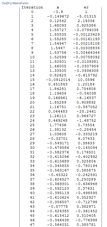
fixedpoint3

The expression $f(x)=0$ can be converted to different forms $x=g(x)$ . For example, assuming $x\neq 0$ :

$0=\sin{5x}+\cos{2x}\Rightarrow 0=\frac{\sin{5x}+\cos{2x}}{x}\Rightarrow x=\frac{\sin{5x}+\cos{2x}}{x}+x$

If this expression is used, the fixed-point iteration method does converge depending on the choice of $x_0$ . For example, setting $x_0=5.0$ gives the estimate for the root $x_6=4.26452$ with the required accuracy:

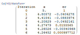View Mathematica Code

Clear[x, g]
x = {5.};
er = {1};
es = 0.001;
MaxIter = 100;
i = 1;
g[x_] := (Sin[5 x] + Cos[2 x])/x + x
While[And[i <= MaxIter, Abs[er[[i]]] > es], xnew = g[x[[i]]]; x = Append[x, xnew]; ernew = (xnew - x[[i]])/xnew; er = Append[er, ernew]; i++];
T = Length[x];
SolutionTable = Table[{i - 1, x[[i]], er[[i]]}, {i, 1, T}];
SolutionTable1 = {"Iteration", "x", "er"};
T = Prepend[SolutionTable, SolutionTable1];
T // MatrixForm

View Python Code

import numpy as np
import pandas as pd

x = [5]
er = [1]
es = 0.001
MaxIter = 100
i = 0
def g(x): return (np.sin(5*x) + np.cos(2*x))/x + x
while i <= MaxIter and abs(er[i]) > es:
  xnew = g(x[i])
  x.append(xnew)
  ernew = (xnew - x[i])/xnew
  er.append(ernew)
  i+=1
SolutionTable = [[i, x[i], er[i]] for i in range(len(x))]
pd.DataFrame(SolutionTable, columns=["Iteration", "x", "er"])

Obviously, unlike the bracketing methods, this open method cannot find a root in a specific interval. The root is a function of the initial guess $x_0$ and the form $x=g(x)$ , but the user has no other way of forcing the root to be within a specific interval. It is very difficult, for example, to use the fixed-point iteration method to find the roots of the expression $0=\sin{5x}+\cos{2x}$ in the interval $[-1,1]$ .

Analysis of Convergence of the Fixed-Point Method

The objective of the fixed-point iteration method is to find the true value $V_t$ that satisfies $V_t=g(V_t)$ . In each iteration we have the estimate $x_{i+1}=g(x_i)$ . Using the mean value theorem, we can write the following expression:

$g(x_i)=g(V_t)+g'(\xi)(x_i-V_t)$

for some $\xi$ in the interval between $x_i$ and the true value $V_t$ . Replacing $g(V_t)$ and $g(x_i)$ in the above expression yields:

$x_{i+1}=V_t+g'(\xi)(x_i-V_t)\Rightarrow x_{i+1}-V_t=g'(\xi)(x_i-V_t)$

The error after iteration $i+1$ is equal to $E_{i+1}=V_t-x_{i+1}$ while that after iteration $i$ is equal to $E_i=V_t-x_i$ . Therefore, the above expression yields:

$E_{i+1}=g'(\xi)E_i$

For the error to reduce after each iteration, the first derivative of $g$ , namely $g'$ , should be bounded by 1 in the region of interest (around the required root):

$|g'(\xi)|< 1$

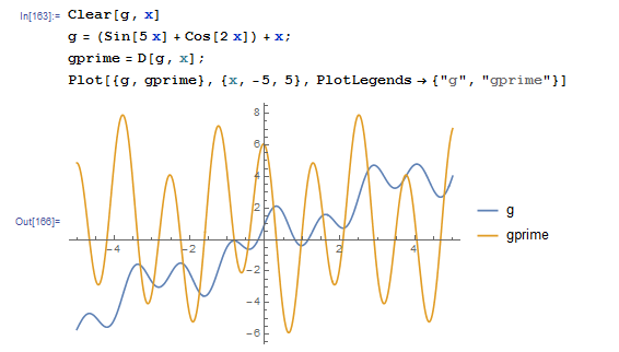
We can now try to understand why, in the previous example, the expression $x=g(x)=\sin{5x}+\cos{2x}+x$ does not converge. When we plot $g(x)$ and $g'(x)$ we see that $g'(x)$ oscillates rapidly with values higher than 1:

fixedpoint5

On the other hand, the expression $x=g(x)=\frac{\sin{5x}+\cos{2x}}{x}+x$ converges for roots that are away from zero. When we plot $g(x)$ and $g'(x)$ we see that the oscillations in $g'(x)$ decrease when $x$ is away from zero and $g'(x)$ is bounded by 1 in some regions:
fixedpoint6

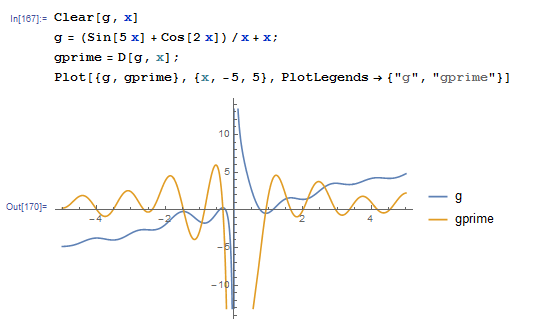
Example

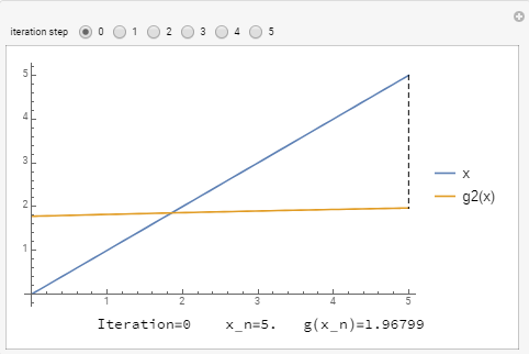
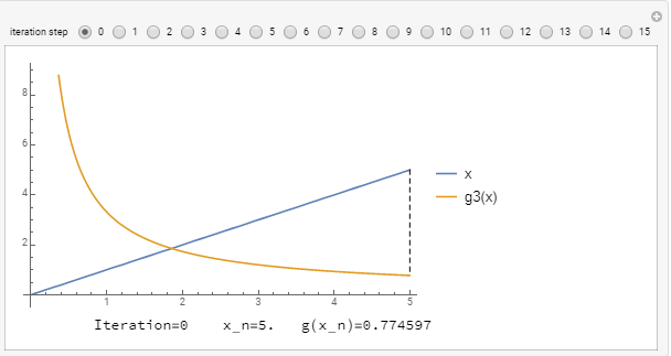
In this example, we will visualize the example of finding the root of the expression $x^4-x-10=0$ . There are three different forms for the fixed-point iteration scheme:

$\begin{split}x&=g_1(x)=\frac{10}{x^3-1}\\x&=g_2(x)=(x+10)^{1/4}\\x&=g_3(x)=\frac{(x+10)^{1/2}}{x}\end{split}$

To visualize the convergence, notice that if we plot the separate graphs of the function $x$ and the function $g(x)$ , then, the root is the point of intersection when $x=g(x)$ . For $g_1(x)$ , the slope $g_1'(x)$ is not bounded by 1 and so, the scheme diverges no matter what $x_0$ is. Here we start with $x_0=2$ :

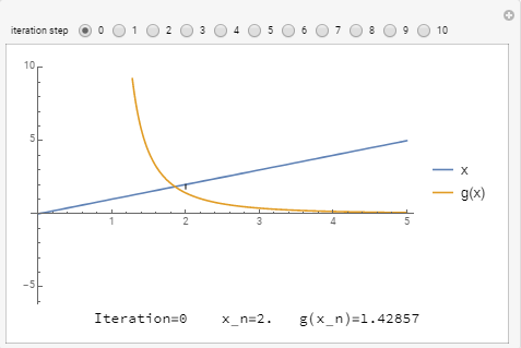
For $g_2(x)$ , the slope $g_2'(x)$ is bounded by 1 and so, the scheme converges really fast no matter what $x_0$ is. Here we start with $x_0=5$ :

For $g_3(x)$ , the slope $g_3'(x)$ is bounded by 1 and so, the scheme converges but slowly. Here we start with $x_0=5$ :

The following is the Mathematica code used to generate one of the tools above:

View Mathematica Code

Manipulate[
 x = {5.};
 er = {1};
 es = 0.001;
 MaxIter = 20;
 i = 1;
 g[x_] := (x + 10)^(1/4);
 While[And[i <= MaxIter, Abs[er[[i]]] > es],xnew = g[x[[i]]]; x = Append[x, xnew]; ernew = (xnew - x[[i]])/xnew;er = Append[er, ernew]; i++];
 T1 = Length[x];
 SolutionTable = Table[{i - 1, x[[i]], er[[i]]}, {i, 1, T1}];
 SolutionTable1 = {"Iteration", "x", "er"};
 T = Prepend[SolutionTable, SolutionTable1];
 LineTable1 = Table[{{T[[i, 2]], T[[i, 2]]}, {T[[i, 2]], g[T[[i, 2]]]}}, {i, 2, n}];
 LineTable2 = Table[{{T[[i + 1, 2]], T[[i + 1, 2]]}, {T[[i, 2]], g[T[[i, 2]]]}}, {i, 2, n - 1}];
 Grid[{{Plot[{x, g[x]}, {x, 0, 5}, PlotLegends -> {"x", "g3(x)"},ImageSize -> Medium, Epilog -> {Dashed, Line[LineTable1], Line[LineTable2]}]}, {Row[{"Iteration=", n - 2, "    x_n=", T[[n, 2]], "   g(x_n)=", g[T[[n, 2]]]}]}}], {n, 2, Length[T], 1}]

View Python Code

import numpy as np
import matplotlib.pyplot as plt
from ipywidgets.widgets import interact

def g(x): return (x + 10)**(1/4)
@interact(n=(2,6,1))
def update(n=1):
  x = [5]
  er = [1]
  es = 0.001
  MaxIter = 20
  i = 0
  while i <= MaxIter and abs(er[i]) > es:
    xnew = g(x[i])
    x.append(xnew)
    ernew = (xnew - x[i])/xnew
    er.append(ernew)
    i+=1
  SolutionTable = [[i, x[i], er[i]] for i in range(len(x))]
  LineTable = [[],[]]
  for i in range(n-1):
    LineTable[0].extend([SolutionTable[i][1], SolutionTable[i][1]])
    LineTable[1].extend([SolutionTable[i][1], g(SolutionTable[i][1])])
  x_val = np.arange(0,5.1,0.1)
  plt.plot(x_val,x_val, label="x")
  plt.plot(x_val,g(x_val), label="g3(x)")
  plt.plot(LineTable[0],LineTable[1],'k--')
  plt.legend(); plt.grid(); plt.show()
  print("Iteration =",n-2," x_n =",round(SolutionTable[n-2][1],5)," g(x_n) =",round(g(SolutionTable[n-2][1]),5))

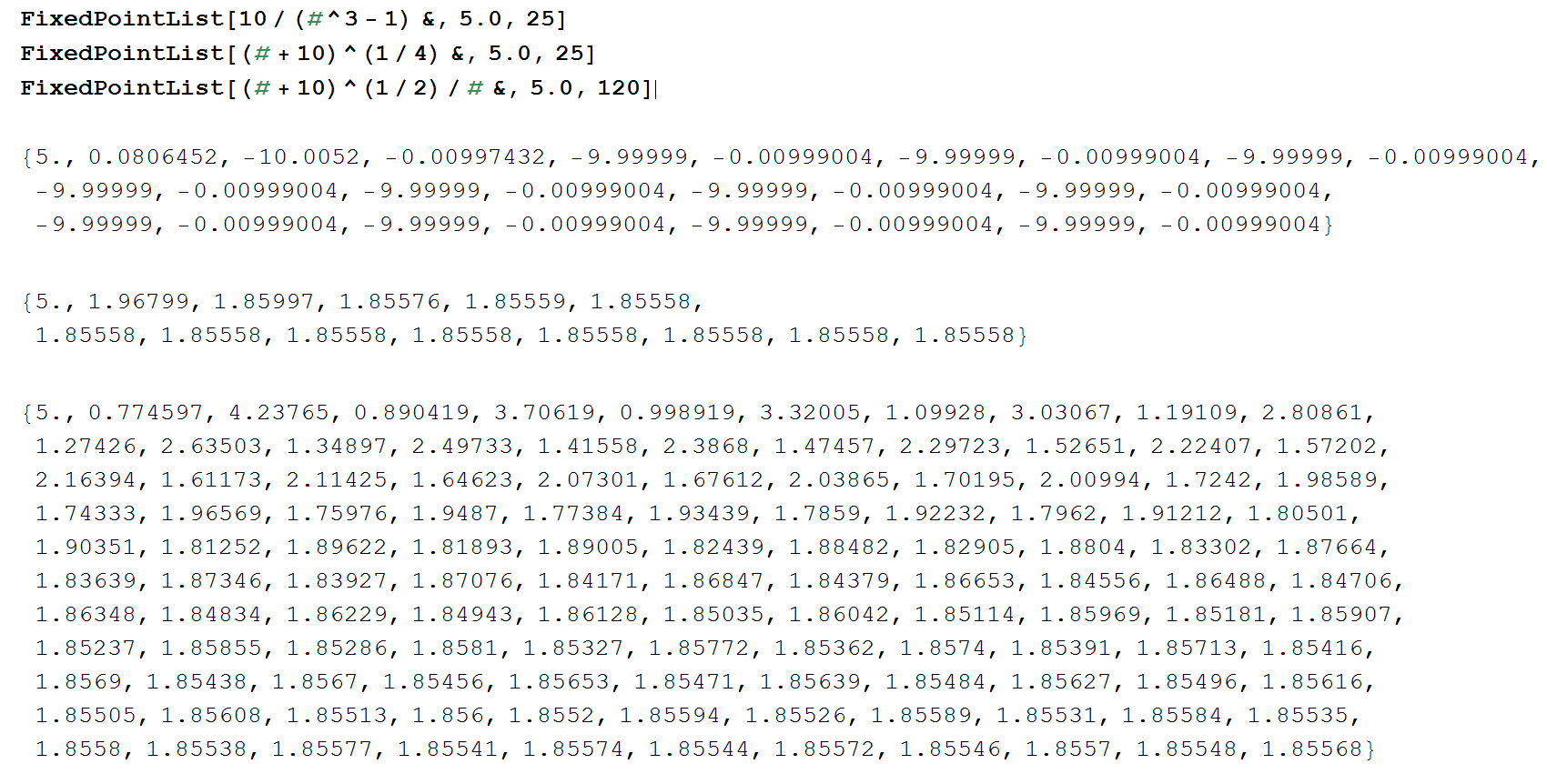
The following shows the output if we use the built-in fixed-point iteration function for each of $g_1$ , $g_2$ , and $g_3$ . $g_1$ oscillates and so, it will never converge. $g_2$ converges really fast (3 to 4 iterations). $g_3$ converges really slow, taking up to 120 iterations to converge.