Engineering at Alberta Courses » Linearization of Nonlinear Relationships

Curve Fitting: Linearization of Nonlinear Relationships

Linearization of Nonlinear Relationships

In the previous two sections, the model function $y$ was formed as a linear combination of functions $f_1,f_2,\cdots,f_m$ and the minimization of the sum of the squares of the differences between the model prediction and the data produced a linear system of equations to solve for the coefficients in the model. In that case $y$ was linear in the coefficients. In certain situations, it is possible to convert nonlinear relationships to a linear form similar to the previous methods. For example, consider the following models $y_{\mbox{exp}}$ , $y_{\mbox{power}}$ , and $y_{\mbox{log}}$ :

$y_{\mbox{exp}}=b_1e^{a_1x}\qquad y_{\mbox{power}}=b_2x^{a_2} \qquad y_{\mbox{log}}=a_3\ln x + b_3$

$y_{\mbox{exp}}$ is an exponential model, $y_{\mbox{power}}$ is a power model, while $y_{\mbox{log}}$ is a logarithmic model. These models are nonlinear in $x$ and the unknown coefficients. However, by taking the natural logarithm of the first two, they can easily be transformed into linear models as follows:

$\ln y_{\mbox{exp}}=a_1 x+\ln b_1 \qquad \ln y_{\mbox{power}}=a_2 \ln x+\ln b_2$

In the first model, the data can be converted to $(x_i,\ln y_i)$ and linear regression can be used to find the coefficients $a_1$ and $\ln b_1$ . For the second model, the data can be converted to $(\ln x_i,\ln y_i)$ and linear regression can be used to find the coefficients $a_2$ , and $\ln b_2$ . The third model can be considered linear after converting the data into the form $(\ln x_i, y_i)$ .

Coefficient of Determination for Nonlinear Relationships

For nonlinear relationships, the coefficient of determination is not a very good measure for how well the data fit the model. See for example this article on the subject. In fact, different software will give different values for $R^2$ . We will use the coefficient of determination for nonlinear relationships defined as:

$R^2=1-\frac{\sum_{i=1}^n\left(y_i-y(x_i)\right)^2}{\sum_{i=1}^n\left(y_i\right)^2}$

which is equal to 1 minus the ratio between the model sum of squares and the total sum of squares of the data. This is consistent with the definition of $R^2$ used in Mathematica for nonlinear models.

Example 1

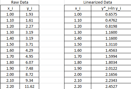
Fit an exponential model to the data: (1,1.93),(1.1,1.61),(1.2,2.27),(1.3,3.19),(1.4,3.19),(1.5,3.71),(1.6,4.29),(1.7,4.95),(1.8,6.07),(1.9,7.48),(2,8.72),(2.1,9.34),(2.2,11.62).

Solution

The exponential model has the form:

$y_{\mbox{exp}}=b_1e^{a_1x}$

This form can be linearized as follows:

$\ln y_{\mbox{exp}}=a_1 x+\ln b_1$

The data needs to be converted to $(x_i,\ln y_i)$ . $y^*$ will be used to designate $\ln y$ . The following Microsoft Excel table shows the raw data, and after conversion to $(x_i,y^*_i)$ .

example 11

The linear regression described above will be used to find the best fit for the model:

$y^*=a^*x+b^*$

with

$\begin{split}a^*&=\frac{n\sum_{i=1}^nx_iy^*_i-\sum_{i=1}^nx_i\sum_{i=1}^ny^*_i}{n\sum_{i=1}^nx_i^2-\left(\sum_{i=1}^nx_i\right)^2}\\b^*&=\frac{\sum_{i=1}^ny^*_i-a^*\sum_{i=1}^nx_i}{n}\end{split}$

The following Microsoft Excel table is used to calculate the various entries in the above equation:

betternumbers1

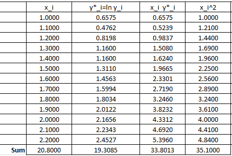
Therefore:

$\begin{split}a^*&=\frac{13\times 33.8013-20.8\times 19.3085}{13\times 35.10-\left(20.8\right)^2}=1.5976\\b^*&=\frac{19.3085-1.5976\times 20.8}{13}=-1.0709\end{split}$

These can be used to calculate the coefficients in the original model:

$a_1=a^*=1.5976 \qquad b_1=e^{b^*}=e^{-1.0709}=0.3427$

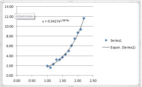
Therefore, the best exponential model based on the least squares of the linearized version has the form:

$y_{\mbox{exp}}=0.3427e^{1.5976x}$

The following Microsoft Excel chart shows the calculated trendline in Excel with the same coefficients:

example 23

It is possible to calculate the coefficient of determination for the linearized version of this model, however, it would only describe how good the linearized model is. For the nonlinear model, we will use the coefficient of determination as described above which requires the following Microsoft Excel table: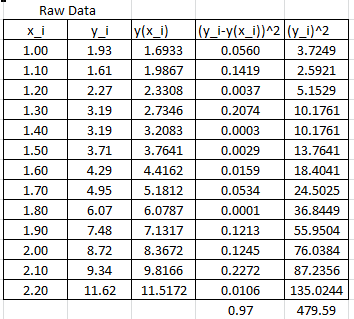
Example25
In this case, the coefficient of determination can be calculated as:

$R^2=1-\frac{\sum_{i=1}^n\left(y_i-y(x_i)\right)^2}{\sum_{i=1}^n\left(y_i\right)^2}=1-\frac{0.97}{479.59}=0.998$

The NonlinearModelFit built-in function in Mathematica can be used to generate the model and calculate its $R^2$ as shown in the code below.

View Mathematica Code

Data = {{1, 1.93}, {1.1, 1.61}, {1.2, 2.27}, {1.3, 3.19}, {1.4, 3.19}, {1.5, 3.71}, {1.6, 4.29}, {1.7, 4.95}, {1.8, 6.07}, {1.9, 7.48}, {2, 8.72}, {2.1, 9.34}, {2.2, 11.62}};
model = NonlinearModelFit[Data, b1*E^(a1*x), {a1, b1}, x]
y = Normal[model]
R2 = model["RSquared"]
Plot[y, {x, 1, 2.2}, Epilog -> {PointSize[Large], Point[Data]}, PlotLegends -> {"Model"}, AxesLabel -> {"x", "y"}, AxesOrigin -> {0, 0} ]

View Python Code

import numpy as np
import matplotlib.pyplot as plt
from scipy.optimize import curve_fit

Data = [[1, 1.93], [1.1, 1.61], [1.2, 2.27], [1.3, 3.19], [1.4, 3.19], [1.5, 3.71], [1.6, 4.29], [1.7, 4.95], [1.8, 6.07], [1.9, 7.48], [2, 8.72], [2.1, 9.34], [2.2, 11.62]]
def f(x, a, b): return a*np.exp(b*x)
coeff, covariance = curve_fit(f, [point[0] for point in Data],
                                 [point[1] for point in Data])
print("coeff: ",coeff)
x_val = np.arange(1,2.2,0.01)
plt.title('%.5fe**(%.5fx)' % tuple(coeff))
plt.plot(x_val, f(x_val, coeff[0], coeff[1]))
plt.scatter([point[0] for point in Data], [point[1] for point in Data], c='k')
plt.xlabel("x"); plt.ylabel("y")
plt.grid(); plt.show()

# R squared
x = np.array([point[0] for point in Data])
y = np.array([point[1] for point in Data])
y_fit = f(x, coeff[0], coeff[1])
ss_res = np.sum((y - y_fit)**2)
ss_tot = np.sum((y - np.mean(y))**2)
r2 = 1 - (ss_res / ss_tot)
print("R Squared: ",r2)

The following link provides the MATLAB codes for implementing the Linearization of nonlinear exponential model.

MATLAB file: File 1 (ex9_4.m)

Example 2

Fit a power model to the data: (1,1.93),(1.1,1.61),(1.2,2.27),(1.3,3.19),(1.4,3.19),(1.5,3.71),(1.6,4.29),(1.7,4.95),(1.8,6.07),(1.9,7.48),(2,8.72),(2.1,9.34),(2.2,11.62).

Solution

The power model has the form:

$y_{\mbox{power}}=b_2x^{a_2}$

This form can be linearized as follows:

$\ln y_{\mbox{power}}=a_2 \ln x+\ln b_2$

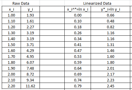
The data needs to be converted to $(\ln x_i,\ln y_i)$ . $y^*$ and $x^*$ will be used to designate $\ln y$ and $\ln x$ respectively. The following Microsoft Excel table shows the raw data, and after conversion to $(x_i^*,y^*_i)$ .

Example b1

The linear regression described above will be used to find the best fit for the model:

$y^*=a^*x^*+b^*$

with

$\begin{split}a^*&=\frac{n\sum_{i=1}^nx_i^*y^*_i-\sum_{i=1}^nx_i^*\sum_{i=1}^ny^*_i}{n\sum_{i=1}^n(x_i^*)^2-\left(\sum_{i=1}^nx_i^*\right)^2}\\b^*&=\frac{\sum_{i=1}^ny^*_i-a^*\sum_{i=1}^nx_i^*}{n}\end{split}$

The following Microsoft Excel table is used to calculate the various entries in the above equation:

betternumbers2

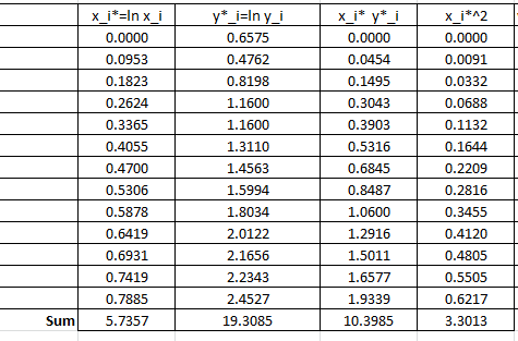
Therefore:

$\begin{split}a^*&=\frac{13\times 10.3985-5.7357\times 19.3085}{13\times 3.3013-\left(5.7357\right)^2}=2.4387\\b^*&=\frac{19.3085-2.4387\times 5.7357}{13}=0.4093\end{split}$

These can be used to calculate the coefficients in the original model:

$a_2=a^*=2.4387 \qquad b_2=e^{b^*}=e^{0.4093}=1.5058$

Therefore, the best power model based on the least squares of the linearized version has the form:

$y_{\mbox{power}}=1.5058x^{2.4387}$

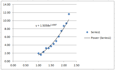
The following Microsoft Excel chart shows the calculated trendline in Excel with the same coefficients:

power1

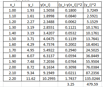
In this case, the coefficient of determination can be calculated as:

$R^2=1-\frac{\sum_{i=1}^n\left(y_i-y(x_i)\right)^2}{\sum_{i=1}^n\left(y_i\right)^2}=1-\frac{3.25}{479.59}=0.9932$

The NonlinearModelFit built-in function in Mathematica can be used to generate a slightly better model with a higher $R^2$ . The following is the corresponding Mathematica output.

Power3

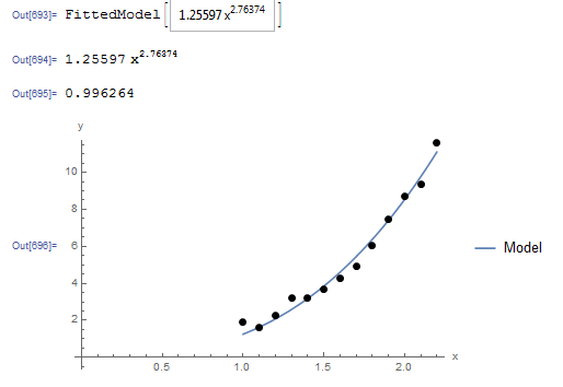
The Mathematica code is shown below.

View Mathematica Code

Data = {{1, 1.93}, {1.1, 1.61}, {1.2, 2.27}, {1.3, 3.19}, {1.4, 3.19}, {1.5, 3.71}, {1.6, 4.29}, {1.7, 4.95}, {1.8, 6.07}, {1.9, 7.48}, {2, 8.72}, {2.1, 9.34}, {2.2, 11.62}};
model = NonlinearModelFit[Data, b1*x^(a1), {a1, b1}, x]
y = Normal[model]
R2 = model["RSquared"]
Plot[y, {x, 1, 2.2}, Epilog -> {PointSize[Large], Point[Data]}, PlotLegends -> {"Model"}, AxesLabel -> {"x", "y"}, AxesOrigin -> {0, 0} ]

View Python Code

import numpy as np
import matplotlib.pyplot as plt
from scipy.optimize import curve_fit

Data = [[1, 1.93], [1.1, 1.61], [1.2, 2.27], [1.3, 3.19], [1.4, 3.19], [1.5, 3.71], [1.6, 4.29], [1.7, 4.95], [1.8, 6.07], [1.9, 7.48], [2, 8.72], [2.1, 9.34], [2.2, 11.62]]
def f(x, a, b): return a*x**b
coeff, covariance = curve_fit(f, [point[0] for point in Data],
                                 [point[1] for point in Data])
print("coeff: ",coeff)
x_val = np.arange(1,2.2,0.01)
plt.title('%.5fx**(%.5f)' % tuple(coeff))
plt.plot(x_val, f(x_val, coeff[0], coeff[1]))
plt.scatter([point[0] for point in Data], [point[1] for point in Data], c='k')
plt.xlabel("x"); plt.ylabel("y")
plt.grid(); plt.show()

# R squared
x = np.array([point[0] for point in Data])
y = np.array([point[1] for point in Data])
y_fit = f(x, coeff[0], coeff[1])
ss_res = np.sum((y - y_fit)**2)
ss_tot = np.sum((y - np.mean(y))**2)
r2 = 1 - (ss_res / ss_tot)
print("R Squared: ",r2)

The following link provides the MATLAB codes for implementing the Linearization of nonlinear power model.

MATLAB files: File 1 (ex9_5.m)

Open Educational Resources

Curve Fitting: Linearization of Nonlinear Relationships

Linearization of Nonlinear Relationships

Coefficient of Determination for Nonlinear Relationships

Example 1

Solution

Example 2

Solution

Lecture Video

Leave a Reply Cancel reply