Engineering at Alberta Courses » Simpson’s Rules

Numerical Integration: Simpson’s Rules

Simpson’s ⅓ Rule

Let $f:[a,b]\rightarrow \mathbb{R}$ . By dividing the interval $[a,b]$ into many subintervals, the Simpson’s 1/3 rule approximates the area under the curve in every subinterval by interpolating between the values of the function at the midpoint and ends of the subinterval, and thus, on each subinterval, the curve to be integrated is a parabola. For simplicity, the width of each subinterval is chosen to be constant and is equal to $2h$ . Let $n$ be the number of intervals with $a=x_0 < x_1 < x_2 < \cdots < x_n=b$ and constant spacing $2h=x_{i}-x_{i-1}$ . On each interval with end points $x_{i-1}$ and $x_i$ , Lagrange polynomials can be used to define the interpolating parabola as follows:

$p_2(x)=f(x_{i-1})\frac{(x-{x_m}_i)(x-x_{i})}{2h^2}+f({x_m}_i)\frac{(x-x_{i-1})(x-x_{i})}{-h^2}+f(x_{i})\frac{(x-x_{i-1})(x-{x_m}_i)}{2h^2}$

where ${x_m}_i$ is the midpoint in the interval $i$ . Integrating the above formula yields:

$\int_{x_{i-1}}^{x_i}\!p_2(x)\,\mathrm{d}x=\frac{h}{3}\left(f(x_{i-1})+4f({x_m}_i)+f(x_{i})\right)$

The Simpson’s 1/3 rule can be implemented as follows:

$\begin{split}I_{S1} & =\int_{a}^b\!f(x)\,\mathrm{d}x\approx \frac{h}{3}\sum_{i=1}^{n}\left(f(x_{i-1})+4f({x_m}_i)+f(x_i)\right)\\&=\frac{h}{3}(f(x_0)+4f({x_m}_1)+2f(x_1)+4f({x_m}_2)+2f(x_2)+\cdots+2f(x_{n-1})+4f({x_m}_n)+f(x_n))\end{split}$

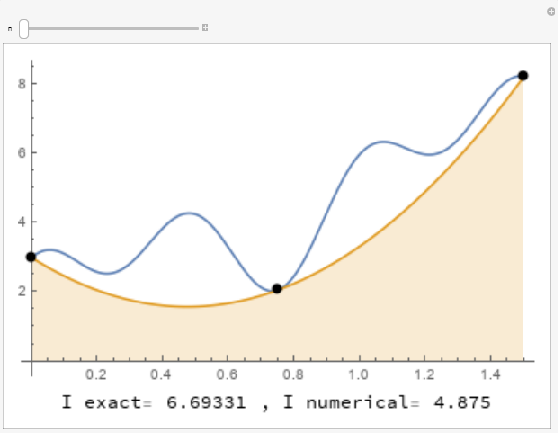
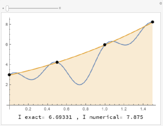
The following tool illustrates the implementation of the Simpson’s 1/3 rule for integrating the function $f:[0,1.5]\rightarrow \mathbb{R}$ defined as:

$f(x)= 2 + 2 x + x^2 + \sin{(2 \pi x)} + \cos{(2 \pi \frac{x}{0.5})}$

Use the slider to see the effect of increasing the number of intervals on the approximation.

The following Mathematica code can be used to numerically integrate any function $f$ on the interval $[a,b]$ using the Simpson’s 1/3 rule.

View Mathematica Code

IS1[f_, a_, b_, n_] := (h = (b - a)/2/n; h/3*Sum[(f[a + (2i - 2)*h] + 4*f[a + (2i - 1)*h]+f[a + (2i)*h]), {i, 1, n}])
f[x_] := 2 + 2 x + x^2 + Sin[2 Pi*x] + Cos[2 Pi*x/0.5];
IS1[f, 0, 1.5, 1.0]
IS1[f, 0, 1.5, 18.0]

View Python Code

import numpy as np
def IS1(f, a, b, n):
  h = (b - a)/2/n
  return h/3*sum([(f(a + (2*i)*h) + 4*f(a + (2*i + 1)*h) + f(a + (2*i + 2)*h)) for i in range(int(n))])
def f(x): return 2 + 2*x + x**2 + np.sin(2*np.pi*x) + np.cos(2*np.pi*x/0.5)
print(IS1(f, 0, 1.5, 1.0))
print(IS1(f, 0, 1.5, 18.0))

The following link provides the MATLAB codes for implementing the Simpson’s 1/3 rule.

MATLAB files: File 1 (simpson13.m)

Error Analysis

One estimate for the upper bound of the error can be derived similar to the derivation of the upper bound of the error in the trapezoidal rule as follows. Given a function $f$ and its interpolating polynomial of degree $n$ ( $p_n(x)$ ), the error term between the interpolating polynomial and the function is given by (See the Mathematical Background section for a proof):

$f(x)=p_n(x)+\frac{f^{n+1}(\xi)}{(n+1)!}\prod_{i=1}^{n+1}(x-x_{i})$

Where $\xi$ is in the domain of the function $f$ . The error in the calculation of the integral of the parabola number $i$ connecting the points $x_{i-1}$ , $x_{m}=\frac{x_{i-1}+x_i}{2}$ , and $x_{i}$ will be estimated based on the above formula assuming $2h=x_i-x_{i-1}$ . Therefore:

$\begin{split}|E_i|&=\left|\int_{x_{i-1}}^{x_i}\! f(x)-p_2(x)\,\mathrm{d}x\right|=\left|\int_{x_{i-1}}^{x_i}\!\frac{f'''(\xi)}{3\times 2}(x-x_{i-1})(x-x_m)(x-x_i)\,\mathrm{d}x\right|\end{split}$

Therefore, the upper bound for the error can be given by:

$|E_i|\leq \max_{\xi\in[x_{i-1},x_i]}\frac{|f'''(\xi)|}{6}\int_{x_{i-1}}^{x_i}\!|(x-x_{i-1})(x-x_m)(x-x_i)|\,\mathrm{d}x=\max_{\xi\in[x_{i-1},x_i]}\frac{|f''(\xi)|h^4}{12}$

If $n$ is the number of subdivisions, where each subdivision has width of $2h$ , i.e., $n(2h)=b-a$ , then:

$|E|=|nE_i|\leq \max_{\xi\in[a,b]}\frac{|f'''(\xi)|nh^4}{12}=\max_{\xi\in[a,b]}\frac{|f'''(\xi)|(b-a)h^3}{24}$

However, it can actually be shown that there is a better estimate for the upper bound of the error. This can be shown using Newton interpolating polynomials through the points $x_{i-1},x_m,x_i,x_{i}+h$ . The reason we add an extra point is going to become apparent when the integration is carried out. The error term between the interpolating polynomial and the function is given by:

$\begin{split}f(x)=&b_1+b_2(x-x_{i-1})+b_3(x-x_{i-1})(x-x_{m})+b_4(x-x_{i-1})(x-x_{m})(x-x_{i})\\&+\frac{f''''(\xi)}{4!}(x-x_{i-1})(x-x_{m})(x-x_{i})(x-x_{i}-h)\end{split}$

where $\xi\in[x_{i-1},x_{i}+h]$ and is dependent on $x$ . The first three terms on the right-hand side are exactly the interpolating parabola passing through the points $f(x_{i-1})$ , $f(x_{m})$ , and $f(x_{i})$ . Therefore, an estimate for the error can be evaluated as:

$\begin{split}|E_i|&=\left|\int_{x_{i-1}}^{x_i}\! f(x)-b_1-b_2(x-x_{i-1})-b_3(x-x_{i-1})(x-x_{m})\,\mathrm{d}x\right|\\&\leq \left|\int_{x_{i-1}}^{x_i}\!b_4(x-x_{i-1})(x-x_{m})(x-x_{i})\,\mathrm{d}x\right|\\&+\max_{\xi\in[x_{i-1},x_{i}+h]}\left|\frac{f''''(\xi)}{4!}\right|\int_{x_{i-1}}^{x_i}\!\left|(x-x_{i-1})(x-x_{m})(x-x_{i})(x-x_{i}-h)\right|\mathrm{d}x\\&\leq 0 + \max_{\xi\in[x_{i-1},x_{i}+h]}\left|\frac{f''''(\xi)}{4!}\right|\frac{4h^5}{15}\\&\leq \max_{\xi\in[x_{i-1},x_{i}+h]}\left|f''''(\xi)\right|\frac{h^5}{90}\end{split}$

The first term on the right-hand side of the inequality is equal to zero. This is because the point $x_m$ is the average of $x_{i-1}$ and $x_i$ , so, integrating that cubic polynomial term yields zero. This was the reason to consider a third-order polynomial instead of a second-order polynomial which allows the error term to be in terms of $h^5$ . If $n$ is the number of subdivisions, where each subdivision has width of $2h$ , i.e., $n(2h)=b-a$ , then:

$|E|=|nE_i|\leq \max_{\xi\in[a,b]}\frac{|f''''(\xi)|nh^5}{90}=\max_{\xi\in[a,b]}\frac{|f''''(\xi)|(b-a)h^4}{180}$

Example

Using the Simpson’s 1/3 rule with $n=2$ , calculate $I_{S1}$ and compare with the exact integral of the function $f(x)=e^x$ on the interval $[0,2]$ . Find the value of $h$ so that the error is less than 0.001.

Solution

It is important to note that $n$ defines the number of intervals on which a parabola is defined. Each interval has a width of $2h$ . Since $n=2$ the spacing $h$ can be calculated as:

$h=\frac{b-a}{2n}=\frac{2-0}{4}=0.5$

Therefore, $x_0=0$ , $x_1=0.5$ , $x_2=1$ , $x_3=1.5$ , and $x_4=2.0$ . The values of the function at these points are given by:

$f(x_0)=e^0=1.00\qquad f(x_1)=e^{0.5}=1.6487 \qquad f(x_2)=e^{1}=2.7183$

$f(x_3)=e^{1.5}=4.4817 \qquad f(x_4)=e^{2}=7.3891$

According to the Simpson’s 1/3 rule we have:

$\begin{split}I_{S1}&=\frac{h}{3}(f(x_0)+4f(x_1)+2f(x_2)+4f(x_3)+f(x_4))\\&=\frac{0.5}{3} (1 + 4\times 1.6487 + 2\times 2.7183 + 4\times 4.4817 + 7.3891) = 6.391\end{split}$

Which is already a very good approximation to the exact value of $I=6.38906$ even though only 2 intervals were used.

Error Bounds

The total error obtained when $h=0.5$ is indeed less than the error bounds obtained by the formula listed above. For $I_{S1}$ , the error in the estimation is bounded by:

$|E|\leq \max_{\xi\in[a,b]}|f''''(\xi)| (b-a)\frac{h^4}{180}=e^{2}(2-0)\frac{0.5^4}{180}=0.0051$

The error evaluated by $\left|I-I_{S1}\right|=|6.38906-6.391|=0.002$ is indeed less than that upper bound. The same formula can be used to find the value of $h$ so that the error is bounded by 0.001:

$e^{2}(2-0)\frac{h^4}{180}=0.001\Rightarrow h=0.33$

Therefore, to guarantee an error less than 0.001 using $I_{S1}$ , the interval will have to be divided into: $\frac{2}{2(0.33)}=3.03\approx 4$ intervals where a parabola is defined on each! In this case, the value of $I_{S1}=6.38919$ and $|E|=|6.38906-6.38919|=0.0001377$ .

Simpson’s ⅜ Rule

Let $f:[a,b]\rightarrow \mathbb{R}$ . By dividing the interval $[a,b]$ into many subintervals, the Simpson’s 3/8 rule approximates the area under the curve in every subinterval by interpolating between the values of the function at the ends of the subinterval and at two intermediate points, and thus, on each subinterval, the curve to be integrated is a cube. For simplicity, the width of each subinterval is chosen to be constant and is equal to $3h$ . Let $n$ be the number of intervals with $a=x_0 < x_1 < x_2 < \cdots < x_n=b$ and constant spacing $3h=x_{i}-x_{i-1}$ with the intermediate points for each interval $i$ as ${x_l}_i=x_{i-1}+h$ and ${x_r}_i=x_{i-1}+2h$ . On each interval with end points $x_{i-1}$ and $x_i$ , Lagrange polynomials can be used to define the interpolating cubic polynomial as follows:

$\begin{split}p_3(x)&=f(x_{i-1})\frac{(x-{x_l}_i)(x-{x_r}_i)(x-x_{i})}{-6h^3}+f({x_l}_i)\frac{(x-x_{i-1})(x-{x_r}_i)(x-x_{i})}{2h^3}\\&+f({x_r}_i)\frac{(x-x_{i-1})(x-{x_l}_i)(x-x_{i})}{-2h^3}+f(x_{i})\frac{(x-x_{i-1})(x-{x_l}_i)(x-{x_r}_i)}{6h^3}\end{split}$

Integrating the above formula yields:

$\int_{x_{i-1}}^{x_i}\!p_3(x)\,\mathrm{d}x=\frac{3h}{8}\left(f(x_{i-1})+3f({x_l}_i)+3f({x_r}_i)+f(x_{i})\right)$

The Simpson’s 3/8 rule can be implemented as follows:

$\begin{split}I_{S2} & =\int_{a}^b\!f(x)\,\mathrm{d}x\approx \frac{3h}{8}\sum_{i=1}^{n}\left(f(x_{i-1})+3f({x_l}_i)+3f({x_r}_i)+f(x_{i})\right)\\&=\frac{3h}{8}(f(x_0)+3f({x_l}_1)+3f({x_r}_1)+2f(x_1)+\cdots+3f({x_r}_n)+f(x_n))\end{split}$

The following tool illustrates the implementation of the Simpson’s 3/8 rule for integrating the function $f:[0,1.5]\rightarrow \mathbb{R}$ defined as:

$f(x)= 2 + 2 x + x^2 + \sin{(2 \pi x)} + \cos{(2 \pi \frac{x}{0.5})}$

Use the slider to see the effect of increasing the number of intervals on the approximation.

The following Mathematica code can be used to numerically integrate any function $f$ on the interval $[a,b]$ using the Simpson’s 3/8 rule.

View Mathematica Code

IS2[f_, a_, b_, n_] := (h = (b - a)/3/n;3 h/8*Sum[(f[a + (3 i - 3)*h] + 3*f[a + (3 i - 2)*h] + 3 f[a + (3 i - 1)*h] + f[a + (3 i)*h]), {i, 1, n}])
f[x_] := 2 + 2 x + x^2 + Sin[2 Pi*x] + Cos[2 Pi*x/0.5];
IS2[f, 0, 1.5, 5]

View Python Code

import numpy as np
def IS2(f, a, b, n):
  h = (b - a)/3/n
  return 3*h/8*sum([(f(a + (3*i)*h) + 3*f(a + (3*i + 1)*h) + 3*f(a + (3*i + 2)*h) + f(a + (3*i + 3)*h)) for i in range(int(n))])
def f(x): return 2 + 2*x + x**2 + np.sin(2*np.pi*x) + np.cos(2*np.pi*x/0.5)
print(IS2(f, 0, 1.5, 5))

The following link provides the MATLAB codes for implementing the Simpson’s 3/8 rule.

MATLAB files: File 1 (simpson38.m)

Error Analysis

The estimate for the upper bound of the error can be derived similar to the derivation of the upper bound of the error in the trapezoidal rule as follows. Given a function $f$ and its interpolating polynomial of degree $n$ ( $p_n(x)$ ), the error term between the interpolating polynomial and the function is given by (See the Mathematical Background section for a proof):

$f(x)=p_n(x)+\frac{f^{n+1}(\xi)}{(n+1)!}\prod_{i=1}^{n+1}(x-x_{i})$

Where $\xi$ is in the domain of the function $f$ . The error in the calculation of the integral of the cubic function number $i$ connecting the points $x_{i-1}$ , ${x_l}_i=x_{i-1}+h$ , ${x_r}_i=x_{i-1}+2h$ , and $x_{i}=x_{i-1}+3h$ will be estimated based on the above formula assuming $3h=x_i-x_{i-1}$ . Therefore:

$\begin{split}|E_i|&=\left|\int_{x_{i-1}}^{x_i}\! f(x)-p_3(x)\,\mathrm{d}x\right|=\left|\int_{x_{i-1}}^{x_i}\!\frac{f''''(\xi)}{4\times 3\times 2}(x-x_{i-1})(x-{x_l}_i)(x-{x_r}_i)(x-x_i)\,\mathrm{d}x\right|\end{split}$

Therefore, the upper bound for the error can be given by:

$|E_i|\leq \max_{\xi\in[x_{i-1},x_i]}\frac{|f''''(\xi)|}{4\times 3 \times 2}\int_{x_{i-1}}^{x_i}\!|(x-x_{i-1})(x-{x_l}_i)(x-{x_r}_i)(x-x_i)|\,\mathrm{d}x=\max_{\xi\in[x_{i-1},x_i]}\frac{|f''''(\xi)|3h^5}{80}$

If $n$ is the number of subdivisions, where each subdivision has width of $3h$ , i.e., $n(3h)=b-a$ , then:

$|E|=|nE_i|\leq \max_{\xi\in[a,b]}\frac{|f''''(\xi)|3nh^5}{80}=\max_{\xi\in[a,b]}\frac{|f''''(\xi)|(b-a)h^4}{80}$

Example

Using the Simpson’s 3/8 rule with $n=1$ , calculate $I_{S2}$ and compare with the exact integral of the function $f(x)=e^x$ on the interval $[0,2]$ . Find the value of $h$ so that the error is less than 0.001.

Solution

It is important to note that $n$ defines the number of intervals on which a cubic polynomial is defined. Each interval has a width of $3h$ . Since $n=1$ the spacing $h$ can be calculated as:

$h=\frac{b-a}{3n}=\frac{2-0}{3}=0.6667$

Therefore, $x_0=0$ , ${x_l}_1=0.6667$ , ${x_r}_1=1.333$ , and $x_1=2.0$ . The values of the function at these points are given by:

$f(x_0)=e^0=1.00\qquad f({x_l}_1)=e^{0.6667}=1.94773$

$f({x_r}_1)=e^{1.333}=3.79367 \qquad f(x_1)=e^{2}=7.3891$

According to the Simpson’s 3/8 rule we have:

$\begin{split}I_{S2}&=\frac{3h}{8}(f(x_0)+3f({x_l}_1)+3f({x_r}_1)+f(x_1))\\&=\frac{3\times 0.6667}{8} (1 + 3\times 1.94773 + 3\times 3.79367 + 7.3891) = 6.403\end{split}$

Which is already a very good approximation to the exact value of $I=6.38906$ even though only 1 interval was used.

Error Bounds

The total error obtained when $h=0.6667$ is indeed less than the error bounds obtained by the formula listed above. For $I_{S2}$ , the error in the estimation is bounded by:

$|E|\leq \max_{\xi\in[a,b]}|f''''(\xi)| (b-a)\frac{h^4}{80}=e^{2}(2-0)\frac{0.6667^4}{80}=0.0365$

The error $|I-I_{S2}|=|6.38906-6.403|=0.014$ is indeed less than that upper bound. The same formula can be used to find the value of $h$ so that the error is bounded by 0.001:

$e^{2}(2-0)\frac{h^4}{80}=0.001\Rightarrow h=0.27125$

Therefore, to guarantee an error less than 0.001 using $I_{S2}$ , the interval will have to be divided into: $\frac{2}{3(0.27125)}=2.46\approx 3$ intervals where a cubic polynomial is defined on each! In this case, the value of $I_{S2}=6.38925$ and $|E|=|6.38906-6.38925|=0.000192$ .