Engineering at Alberta Courses

Piecewise Interpolation: Introduction

Introduction

In the previous section, it was shown that when the order of the interpolating polynomial increases — which is natural when there is a large number of data points — the interpolating polynomial function can highly oscillate or fluctuate between the data points. With a large number of data points, it is better to keep the order of interpolation low. This can be done using piecewise interpolation using splines. Splines are polynomials on subintervals that are connected with a specified degree of continuity. The order of the polynomials is not associated with the number of data points in this case, so, we can have $k$ data points, and use a spline of degree $n$ where $k>>n$ . Assuming $k$ data points $(x_1,y_1), (x_2,y_2),\cdots,(x_k,y_k)$ such that $x_1<x_2<\cdots<x_k$ , a spline function $y$ of degree $n$ satisfies the following:

On each subinterval $\left[ x_i,x_{i+1} \right)$ , $y$ is a polynomial of degree $n$
The derivatives of $y$ up to and including the $n-1$ derivative are continuous on the domain $[x_1,x_k]$ .

The data points, when chosen such that the spline function passes through them, are called knots. For example, a spline of degree 0 is a piecewise constant function constructed by simply assuming $y$ to have a constant value on any subinterval $\left[x_i,x_{i+1}\right)$ (Figure 1). A spline of degree 1 is a piecewise linear (piecewise affine) function constructed by connecting a straight line between every two data points (Figure 1). A spline of degree 2 is a piecewise quadratic function on each subinterval. The first derivative exists and is continuous, but it is not smooth. As shown in Figure 2, the first derivative is a broken line at the knots and thus the derivatives at the knots do not exist. A spline of degree 3 is a piecewise cubic function on each subinterval. The first and second derivatives are continuous functions. The second derivative is not smooth. Figure 1 shows the resulting 0 order, linear, quadratic, and cubic spline interpolating functions for the data points generated by the Runge function described in the previous section. Figure 2 on the other hand shows the generated derivatives. The 0 order spline function gives a zero derivative everywhere. The linear spline function has derivatives that are constant on each subinterval. The quadratic spline gives derivatives that are not smooth at the data points. The cubic spline provides smooth derivatives that are very close to the actual derivative of the Runge function that was used to generate the data!

The chosen order of the spline function depends on the accuracy sought. Linear splines can provide acceptable interpolation between the knots. However, their derivatives are constant. Linear splines are very useful when the data points are very close to each other, and there is no interest in their derivatives. Quadratic and cubic splines provide very smooth interpolation of the data points. However, the derivatives of the cubic splines are “smoother” than the quadratic splines. The choice of the spline order depends on the oscillatory nature of the data points to be interpolated.

The “Interpolation” built-in function generates an interpolation function through the data. To choose splines, the option: Method->”Spline” has to be specified as well as the interpolation order. The following code generates the 0 order, linear, quadratic, and cubic spline functions through the data points of the Runge function shown in the previous section. The code also compares the first derivatives of the spline functions with the actual first derivative of the Runge function.

View Mathematica Code

Data = {{-1, 0.038}, {-0.8, 0.058}, {-0.60, 0.10}, {-0.4, 0.20}, {-0.2, 0.50}, {0, 1}, {0.2, 0.5}, {0.4, 0.2}, {0.6, 0.1}, {0.8, 0.058}, {1, 0.038}};
y0 = Interpolation[Data, Method -> "Spline", InterpolationOrder -> 0];
y1 = Interpolation[Data, Method -> "Spline", InterpolationOrder -> 1];
y2 = Interpolation[Data, Method -> "Spline", InterpolationOrder -> 2];
y3 = Interpolation[Data, Method -> "Spline", InterpolationOrder -> 3];
yactual = 1/(1 + 25 x^2);
a = Plot[{y0[x], yactual}, {x, -1, 1},Epilog -> {PointSize[Large], Point[Data]}, AxesLabel -> {"x", "y0"}, ImageSize -> Medium, PlotRange -> All, PlotLegends -> {"y0", "yactual"}, PlotLabel -> "0 order splines"];
b = Plot[{y1[x], yactual}, {x, -1, 1},Epilog -> {PointSize[Large], Point[Data]},AxesLabel -> {"x", "y1"}, ImageSize -> Medium, PlotRange -> All,PlotLegends -> {"y1", "yactual"}, PlotLabel -> "Linear splines"];
c = Plot[{y2[x], yactual}, {x, -1, 1},Epilog -> {PointSize[Large], Point[Data]},AxesLabel -> {"x", "y2"}, ImageSize -> Medium, PlotRange -> All, PlotLegends -> {"y2", "yactual"}, PlotLabel -> "Quadratic splines"];
d = Plot[{y3[x], yactual}, {x, -1, 1},Epilog -> {PointSize[Large], Point[Data]},AxesLabel -> {"x", "y3"}, ImageSize -> Medium, PlotRange -> All, PlotLegends -> {"y3", "yactual"}, PlotLabel -> "Cubic splines"];
Grid[{{a, b}, {c, d}}]
y0prime = D[y0[x], x];
y1prime = D[y1[x], x];
y2prime = D[y2[x], x];
y3prime = D[y3[x], x];
yactualprime = D[yactual, x];
a = Plot[{y0prime, yactualprime}, {x, -1, 1},Epilog -> {PointSize[Large], Point[Data]}, AxesLabel -> {"x", "y0"}, ImageSize -> Medium, PlotRange -> All, PlotLegends -> {"y0'", "y'actual"}, PlotLabel -> "Derivative of 0 order splines"];
b = Plot[{y1prime, yactualprime}, {x, -1, 1},Epilog -> {PointSize[Large], Point[Data]},AxesLabel -> {"x", "y1"}, ImageSize -> Medium, PlotRange -> All,PlotLegends -> {"y1'", "y'actual"}, PlotLabel -> "Linear splines"];
c = Plot[{y2prime, yactualprime}, {x, -1, 1},Epilog -> {PointSize[Large], Point[Data]},AxesLabel -> {"x", "y2"}, ImageSize -> Medium, PlotRange -> All,PlotLegends -> {"y2'", "y'actual"}, PlotLabel -> "Quadratic splines"];
d = Plot[{y3prime, yactualprime}, {x, -1, 1},Epilog -> {PointSize[Large], Point[Data]}, AxesLabel -> {"x", "y3"}, ImageSize -> Medium, PlotRange -> All,PlotLegends -> {"y3'", "y'actual"}, PlotLabel -> "Cubic splines"];
Grid[{{a, b}, {c, d}}]

View Python Code

import numpy as np
import matplotlib.pyplot as plt
from scipy.misc import derivative
from scipy.interpolate import interp1d

Data = [[-1, -0.8, -0.60, -0.4, -0.2, 0, 0.2, 0.4, 0.6, 0.8, 1,],[0.038, 0.058, 0.10, 0.20, 0.50, 1, 0.5, 0.2, 0.1, 0.058, 0.038]]
x = np.linspace(-0.99,0.99)
def y(x): return 1/(1 + 25*x**2)

y0 = interp1d(Data[0], Data[1], kind='zero')
y1 = interp1d(Data[0], Data[1], kind='linear')
y2 = interp1d(Data[0], Data[1], kind='quadratic')
y3 = interp1d(Data[0], Data[1], kind='cubic')
yactual = y(x)

plt.title("0 order splines")
plt.xlabel("x"); plt.ylabel("y0")
plt.scatter(Data[0], Data[1], c='k')
plt.plot(x, y0(x), label="y0")
plt.plot(x, yactual, label="yactual")
plt.legend(); plt.grid(); plt.show()

plt.title("Linear splines")
plt.xlabel("x"); plt.ylabel("y1")
plt.scatter(Data[0], Data[1], c='k')
plt.plot(x, y1(x), label="y1")
plt.plot(x, yactual, label="yactual")
plt.legend(); plt.grid(); plt.show()

plt.title("Quadratic splines")
plt.xlabel("x"); plt.ylabel("y2")
plt.scatter(Data[0], Data[1], c='k')
plt.plot(x, y2(x), label="y2")
plt.plot(x, yactual, label="yactual")
plt.legend(); plt.grid(); plt.show()

plt.title("Cubic splines")
plt.xlabel("x"); plt.ylabel("y3")
plt.scatter(Data[0], Data[1], c='k')
plt.plot(x, y3(x), label="y3")
plt.plot(x, yactual, label="yactual")
plt.legend(); plt.grid(); plt.show()

y0prime = [derivative(y0,i,dx=1e-6) for i in x]
y1prime = [derivative(y1,i,dx=1e-6) for i in x]
y2prime = [derivative(y2,i,dx=1e-6) for i in x]
y3prime = [derivative(y3,i,dx=1e-6) for i in x]
yactualprime = [derivative(y,i,dx=1e-6) for i in x]

plt.title("Derivative of 0 order splines")
plt.xlabel("x"); plt.ylabel("y0")
plt.scatter(Data[0], Data[1], c='k')
plt.plot(x, y0prime, label="y0'")
plt.plot(x, yactualprime, label="y'actual")
plt.legend(); plt.grid(); plt.show()

plt.title("Derivative of Linear splines")
plt.xlabel("x"); plt.ylabel("y1")
plt.scatter(Data[0], Data[1], c='k')
plt.plot(x, y1prime, label="y1'")
plt.plot(x, yactualprime, label="y'actual")
plt.legend(); plt.grid(); plt.show()

plt.title("Derivative of Quadratic splines")
plt.xlabel("x"); plt.ylabel("y2")
plt.scatter(Data[0], Data[1], c='k')
plt.plot(x, y2prime, label="y2'")
plt.plot(x, yactualprime, label="y'actual")
plt.legend(); plt.grid(); plt.show()

plt.title("Derivative of Cubic splines")
plt.xlabel("x"); plt.ylabel("y3")
plt.scatter(Data[0], Data[1], c='k')
plt.plot(x, y3prime, label="y3'")
plt.plot(x, yactualprime, label="y'actual")
plt.legend(); plt.grid(); plt.show()

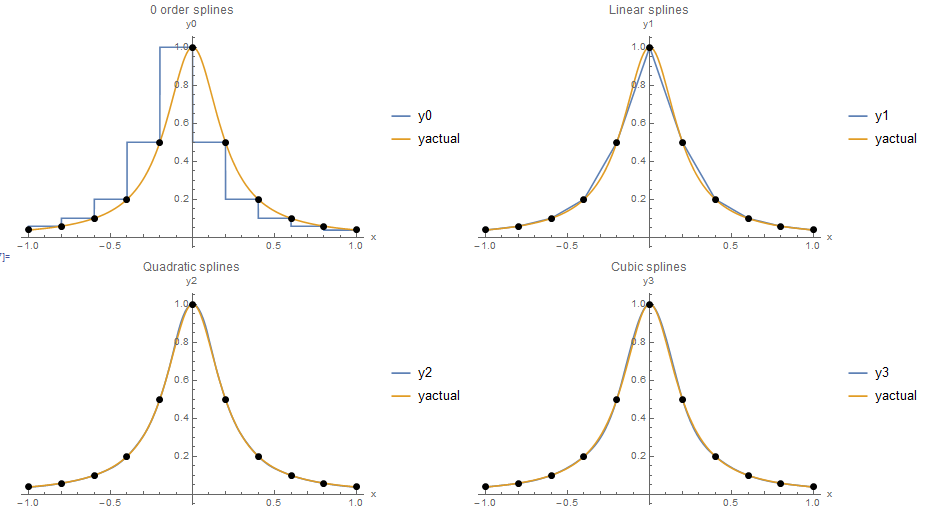
Figure 1. Piecewise interpolation using: 0 order, linear, quadratic, and cubic splines

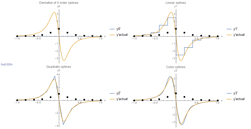
Figure 2. The derivatives of piecewise interpolation using 0 order, linear, quadratic, and cubic splines. The derivative of the 0 order splines is the zero function.

Open Educational Resources

Piecewise Interpolation: Introduction

Introduction

Lecture Video

Leave a Reply Cancel reply