Engineering at Alberta Courses

Open Methods: Secant Method

The Method

The secant method is an alternative to the Newton-Raphson method by replacing the derivative $f'(x)$ with its finite-difference approximation. The secant method thus does not require the use of derivatives especially when $f(x)$ is not explicitly defined. In certain situations, the secant method is preferable over the Newton-Raphson method even though its rate of convergence is slightly less than that of the Newton-Raphson method. Consider the problem of finding the root of the function $f(x)=0$ . Starting with the Newton-Raphson equation and utilizing the following approximation for the derivative $f'(x_{i})$ :

$f'(x_i)=\frac{f(x_i)-f(x_{i-1})}{x_i-x_{i-1}}$

the estimate for iteration $i+1$ can be computed as:

$x_{i+1}=x_i-f(x_i)\frac{x_i-x_{i-1}}{f(x_i)-f(x_{i-1})}$

Obviously, the secant method requires two initial guesses $x_0$ and $x_1$ .

Example

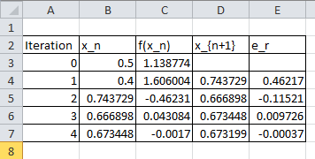
As an example, let’s consider the function $f(x)=\sin{5x}+\cos{2x}$ . Setting the maximum number of iterations $N=100$ , $\varepsilon_s=0.0005$ , $x_0=0.5$ , and $x_1=0.4$ , the following is the Microsoft Excel table produced:
secant1

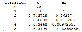
The Mathematica code below can be used to program the secant method with the following output:
secant2

View Mathematica Code

f[x_] := Sin[5 x] + Cos[2 x];
xtable = {0.5, 0.4};
er = {1,1};
es = 0.0005;
MaxIter = 100;
i = 2;
While[And[i <= MaxIter, Abs[er[[i]]] > es], xnew = xtable[[i]] - (f[xtable[[i]]]) (xtable[[i]] - xtable[[i - 1]])/(f[xtable[[i]]] -f[xtable[[i - 1]]]); xtable = Append[xtable, xnew];  ernew = (xnew - xtable[[i]])/xnew; er = Append[er, ernew]; i++];
T = Length[xtable];
SolutionTable = Table[{i - 1, xtable[[i]], er[[i]]}, {i, 1, T}];
SolutionTable1 = {"Iteration", "x", "er"};
T = Prepend[SolutionTable, SolutionTable1];
T // MatrixForm

View Python Code

import numpy as np
import pandas as pd

def f(x): return np.sin(5*x) + np.cos(2*x)
xtable = [0.5, 0.4]
er = [1,1]
es = 0.0005
MaxIter = 100
i = 1
while i <= MaxIter and abs(er[i]) > es:
  xnew = xtable[i] - (f(xtable[i]))*(xtable[i] - xtable[i - 1])/(f(xtable[i]) -f(xtable[i - 1]))
  xtable.append(xnew)
  ernew = (xnew - xtable[i])/xnew
  er.append(ernew)
  i+=1
SolutionTable = [[i, xtable[i], er[i]] for i in range(len(xtable))]
pd.DataFrame(SolutionTable, columns=["Iteration", "x", "er"])

The following code runs the Secant method to find the root of a function $f(x)$ with two initial guesses $x_0$ and $x_1$ . The value of the estimate and approximate relative error at each iteration is displayed in the command window. Additionally, two plots are produced to visualize how the iterations and the errors progress. The program waits for a keypress between each iteration to allow you to visualize the iterations in the figure. Call the function with secant(@(x) f(x), x0, x1). For example try secant(@(x) sin(5.*x)+cos(2.*x),0.5,0.4)

MATLAB file Download

Convergence Analysis of the Secant Method

The $i+1$ estimate in the secant method is obtained as follows:

$x_{i+1}=x_i-f(x_i)\frac{x_i-x_{i-1}}{f(x_i)-f(x_{i-1})}$

Multiplying both sides by -1 and adding the true value of the root $x_t$ where $f(x_t)=0$ for both sides yields:

$x_t-x_{i+1}=x_t-x_i+f(x_i)\frac{x_i-x_{i-1}}{f(x_i)-f(x_{i-1})}$

Using algebraic manipulations:

$\begin{split} x_t-x_{i+1}&=\frac{(x_t-x_i)(f(x_i)-f(x_{i-1}))+f(x_i)(x_i-x_{i-1})}{f(x_i)-f(x_{i-1})}\\ &=\frac{f(x_i)(x_t-x_{i-1})-f(x_{i-1})(x_t-x_i)}{f(x_i)-f(x_{i-1})}\\ &=(x_t-x_{i-1})(x_t-x_i)\frac{\frac{f(x_i)}{x_t-x_i}-\frac{f(x_{i-1})}{x_t-x_{i-1}}}{f(x_i)-f(x_{i-1})} \end{split}$

Using the Mean Value Theorem, the denominator on the right-hand side can be replaced with:

$f(x_i)=f(x_{i-1})+f'(\zeta)(x_i-x_{i-1})$

for some $\zeta$ between $x_i$ and $x_{i-1}$ . Therefore,

$x_t-x_{i+1}=(x_t-x_{i-1})(x_t-x_i)\frac{\frac{f(x_i)}{x_t-x_i}-\frac{f(x_{i-1})}{x_t-x_{i-1}}}{f'(\zeta)(x_i-x_{i-1})}$

Using Taylor’s theorem for $f(x_{i-1})$ and $f(x_i)$ around $x_t$ we get:

$\begin{split} \frac{f(x_i)}{x_t-x_i}=f'(x_t)+\frac{f''(\xi_1)}{2}{(x_t-x_i)}\\ \frac{f(x_i)}{x_t-x_{i-1}}=f'(x_t)+\frac{f''(\xi_2)}{2}{(x_t-x_{i-1})} \end{split}$

for some $\xi_1$ between $x_i$ and $x_t$ and some $\xi_2$ between $x_{i-1}$ and $x_t$ . Using the above expressions we can reach the equation:

$x_t-x_{i+1}=(x_t-x_{i-1})(x_t-x_i)\frac{\frac{f''(\xi_1)}{2}{(x_t-x_i)}-\frac{f''(\xi_2)}{2}{(x_t-x_{i-1})}}{f'(\zeta)(x_i-x_{i-1})}$

$\xi_1$ and $\xi_2$ can be assumed to be identical and equal to $\xi$ , therefore:

$\begin{split} x_t-x_{i+1}&=(x_t-x_{i-1})(x_t-x_i)\frac{\frac{f''(\xi)}{2}{(x_t-x_i-x_t+x_{i-1})}}{f'(\zeta)(x_i-x_{i-1})}\\ &=(x_t-x_{i-1})(x_t-x_i)\frac{-f''(\xi)}{2f'(\zeta)} \end{split}$

Therefore:

(1) $\begin{equation*} E_{i+1}=E_{i}E_{i-1}\left(\frac{-f''(\xi)}{2f'(\zeta)}\right) \end{equation*}$

Comparing the convergence equation of the Newton Raphson method with 1 shows that the convergence in the secant method is not quite quadratic. To find the order of convergence, we need to solve the following equation for a positive $p$ and $C$ :

$|E_{i+1}|=C|E_{i}|^p$

Substituting into equation 1 yields:

$C|E_{i}|^p=|E_{i}||E_{i-1}|\bigg{|}\frac{-f''(\xi)}{2f'(\zeta)}\bigg{|}\Rightarrow E_{i}=\left|\frac{-f''(\xi)}{2Cf'(\zeta)}\right|^{\frac{1}{p-1}}|E_{i-1}|^{\frac{1}{p-1}}$

But we also have:

$|E_{i}|=C|E_{i-1}|^p$

Therefore: $p=\frac{1}{p-1}$ . This equation is called the golden ratio and has the positive solution for $p$ :

$p=\frac{\sqrt{5}+1}{2}\approx 1.618034$

while

$C=\left|\frac{-f''(\xi)}{2f'(\zeta)}\right|^{p-1}=\left|\frac{-f''(\xi)}{2f'(\zeta)}\right|^{0.618034}$

implying that the error convergence is not quadratic but rather:

$E_{i+1}\propto E_i^{1.618034}$

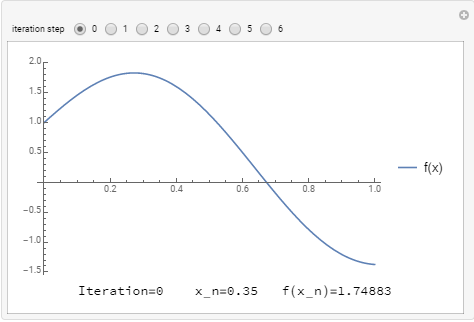
The following tool visualizes how the secant method converges to the true solution using two initial guesses. Using $\varepsilon_s=0.0005$ , $x_0=0.35$ , $x_1=0.4$ , and solving for the root of $f(x)=\sin[5x]+\cos[2x]=0$ yields $x_6=0.6732$ .

The following Mathematica Code was utilized to produce the above tool:

View Mathematica Code

Manipulate[
 f[x_] := x^3 - x + 3;
 f[x_] := Sin[5 x] + Cos[2 x];
 xtable = {-0.5, -0.6};
 xtable = {0.35, 0.4};
 er = {1, 1};
 es = 0.0005;
 MaxIter = 100;
 i = 2;
 While[And[i <= MaxIter, Abs[er[[i]]] > es], xnew = xtable[[i]] - (f[xtable[[i]]]) (xtable[[i]] - xtable[[i-1]])/(f[xtable[[i]]] -f[xtable[[i - 1]]]); xtable = Append[xtable, xnew];  ernew = (xnew - xtable[[i]])/xnew; er = Append[er, ernew]; i++];
 T = Length[xtable];
 SolutionTable = Table[{i - 1, xtable[[i]], er[[i]]}, {i, 1, T}];
 SolutionTable1 = {"Iteration", "x", "er"};
 T = Prepend[SolutionTable, SolutionTable1];
 T // MatrixForm;
 If[n > 3,
  (LineTable1 = {{T[[n - 2, 2]], 0}, {T[[n - 2, 2]], f[T[[n - 2, 2]]]}, {T[[n - 1, 2]], f[T[[n - 1, 2]]]}, {T[[n, 2]], 0}};
   LineTable2 = {{T[[n - 1, 2]], 0}, {T[[n - 1, 2]], f[T[[n - 1, 2]]]}}), LineTable1 = {{}}; LineTable2 = {{}}];
 Grid[{{Plot[f[x], {x, 0, 1}, PlotLegends -> {"f(x)"}, ImageSize -> Medium, Epilog -> {Dashed, Line[LineTable1], Line[LineTable2]}]}, {Row[{"Iteration=", n - 2, "    x_n=", T[[n, 2]], "   f(x_n)=", f[T[[n, 2]]]}]}}], {n, 2, 8, 1}]

View Python Code

import numpy as np
import sympy as sp
import pandas as pd
import matplotlib.pyplot as plt
from ipywidgets.widgets import interact

def f(x): return sp.sin(5*x) + sp.cos(2*x)
xtable = [-0.5, -0.6]
xtable = [0.35, 0.4]
er = [1, 1]
es = 0.0005
MaxIter = 100
i = 1
while i <= MaxIter and abs(er[i]) > es:
  xnew = xtable[i] - (f(xtable[i]))*(xtable[i] - xtable[i-1])/(f(xtable[i]) -f(xtable[i - 1]))
  xtable.append(xnew)
  ernew = (xnew - xtable[i])/xnew
  er.append(ernew)
  i+=1
SolutionTable = [[i, xtable[i], er[i]] for i in range(len(xtable))]
display(pd.DataFrame(SolutionTable, columns=["Iteration", "x", "er"]))

@interact(n=(2,8,1))
def update(n=2):
  LineTable1 = [[],[]]
  LineTable2 = [[],[]]
  if n > 3:
    LineTable1[0] = [SolutionTable[n - 4][1], SolutionTable[n - 4][1], 
                     SolutionTable[n - 3][1], SolutionTable[n-2][1]]
    LineTable1[1] = [0, f(SolutionTable[n - 4][1]), f(SolutionTable[n - 3][1]), 0]
    LineTable2[0] = [SolutionTable[n - 3][1], SolutionTable[n - 3][1]]
    LineTable2[1] = [0, f(SolutionTable[n - 3][1])]

  x_val = np.arange(0,1.1,0.03)
  y_val = np.sin(5*x_val) + np.cos(2*x_val)
  plt.plot(x_val,y_val, label="f(x)")
  plt.plot(LineTable1[0],LineTable1[1],'k--')
  plt.plot(LineTable2[0],LineTable2[1],'k--')
  plt.xlim(0,1,1); plt.ylim(-2,2)
  plt.legend(); plt.grid(); plt.show()
  print("Iteration =",n-2," x_n =",round(SolutionTable[n-2][1],5)," f(x_n) =",round(f(SolutionTable[n-2][1]),5))

Open Educational Resources

Open Methods: Secant Method

The Method

Example

Convergence Analysis of the Secant Method

Lecture video

Leave a Reply Cancel reply