
Numerical Integration: Introduction
Introduction
Integrals arise naturally in the fields of engineering to describe quantities that are functions of infinitesimal data. For example, if the velocity of a moving object for a particular period of time is known, then the change of position of the moving object can be estimated by summing the velocity at discrete time points multiplied by the corresponding time intervals between the discrete points. The accuracy of the change in position can be increased by decreasing the number of discrete time points, i.e., by reducing the time intervals between the discrete points. The formal definition of an integral of a function ![f:[a,b]\rightarrow \mathbb{R}](https://engcourses-uofa.ca/wp-content/ql-cache/quicklatex.com-602dc0a5221796cd029651364476c9ef_l3.png "Rendered by QuickLaTeX.com") is the signed area of the region under the curve
is the signed area of the region under the curve  between the points
  and
and  . The definite integral is denoted by:
![\[\int_{a}^b\!f(x)\,\mathrm{d}x\]](https://engcourses-uofa.ca/wp-content/ql-cache/quicklatex.com-f1a078182b151fa82f3d59313835dc89_l3.png "Rendered by QuickLaTeX.com")
Fundamental Theorem of Calculus
The fundamental theorem of calculus links the concepts of integration and differentiation; roughly speaking, they are the converse of each other. The fundamental theorem of calculus can be stated as follows:
Part I
Let be continuous, and let ![F:[a,b]\rightarrow \mathbb{R}](https://engcourses-uofa.ca/wp-content/ql-cache/quicklatex.com-8f15d39360fb368268c0a775591abd15_l3.png "Rendered by QuickLaTeX.com") be the function defined such that
be the function defined such that ![\forall x\in[a,b]](https://engcourses-uofa.ca/wp-content/ql-cache/quicklatex.com-ee63298b0bb6f908aa2b79bd957b11dc_l3.png "Rendered by QuickLaTeX.com") :
:
![\[F(x)=\int_{a}^x\!f(x)\,\mathrm{d}x\]](https://engcourses-uofa.ca/wp-content/ql-cache/quicklatex.com-6d4604e50cb92dc49d5aaff075bf6fd3_l3.png "Rendered by QuickLaTeX.com")
then,  is uniformly continuous on
 ![[a,b]](https://engcourses-uofa.ca/wp-content/ql-cache/quicklatex.com-1f90ba537767823131bb8d396cdc5a9c_l3.png "Rendered by QuickLaTeX.com") , is differentiable on
, is differentiable on  , and
, and  is the derivative of (also stated as is the antiderivative of ):
![\[\frac{\mathrm{d}F}{\mathrm{d}x}=f(x)\]](https://engcourses-uofa.ca/wp-content/ql-cache/quicklatex.com-e5d9d1e3261657a49cec55bffa4e2db6_l3.png "Rendered by QuickLaTeX.com")
In other words, the first part asserts that if is continuous on the interval , then, an antiderivative always exists; is the derivative of a function that can be defined as  with
with ![x\in[a,b]](https://engcourses-uofa.ca/wp-content/ql-cache/quicklatex.com-7bdc9e9b79b72dde0a30288760e0fe60_l3.png "Rendered by QuickLaTeX.com") .
.
Part II
Let and be two continuous functions such that  (i.e., is the derivative of , or is an antiderivative of ), then:
![\[\int_{a}^b\!f(x)\,\mathrm{d}x=F(b)-F(a)\]](https://engcourses-uofa.ca/wp-content/ql-cache/quicklatex.com-0970c3ed84318d996768ac1a2574611c_l3.png "Rendered by QuickLaTeX.com")
The second part states that if has an antiderivative , then can be used to calculate the definite integral of on the interval .
For visual proofs of the fundamental theorem of calculus, check out this page.
Numerical Integration
The fundamental theorem of calculus allows the calculation of  using the antiderivative of . However, if the antiderivative is not available, a numerical procedure can be employed to calculate the integral or the area under the curve. Historically, the term “Quadrature” was used to mean calculating areas. For example, the Gauss numerical integration scheme that will be studied later is also called the Gauss quadrature. The basic problem in numerical integration is to calculate an approximate solution to the definite integral of a function
 ![f:[a,b]](https://engcourses-uofa.ca/wp-content/ql-cache/quicklatex.com-f9ef6059ed642d0a774671c54562f008_l3.png "Rendered by QuickLaTeX.com") .
.
Riemann Integral
One of the early definitions of the integral of a function is the limit:
![\[\int_{a}^b\!f(x)\,\mathrm{d}x=\lim_{\max{\Delta x_k}\rightarrow 0 } \sum_{k=1}^n f(x_k^*)\Delta x_k\]](https://engcourses-uofa.ca/wp-content/ql-cache/quicklatex.com-b9ed750bade02ab57dda38c6c8ec0175_l3.png "Rendered by QuickLaTeX.com")
where  ,
,  , and
, and  is an arbitrary point such that
 ![x_k^*\in [x_k,x_{k+1}]](https://engcourses-uofa.ca/wp-content/ql-cache/quicklatex.com-1c640bcf7e39a83f233f2cdbba32b682_l3.png "Rendered by QuickLaTeX.com") . If
. If  is the sum of the areas of vertical rectangles arranged next to each other and whose top sides touch the function at arbitrary points, then, the Riemann integral is the limit of this sum as the maximum width of the vertical rectangles approaches zero. A function is “Riemann integrable” if the limit above (the limit of ) exists as the width of the rectangles gets smaller and smaller. In this course, we are always dealing with continuous functions. For continuous functions, the limit always exists and thus, all continuous functions are “Riemann integrable”.
Newton-Cotes Formulas
The Newton-Cotes formulas rely on replacing the function or tabulated data with an interpolating polynomial that is easy to integrate. In this case, the required integral is evaluated as:
![\[I=\int_{a}^b\!f(x)\,\mathrm{d}x\approx \int_{a}^b\!f_n(x)\,\mathrm{d}x \]](https://engcourses-uofa.ca/wp-content/ql-cache/quicklatex.com-b97f7c1084fcb520a2a8f5f52a214463_l3.png "Rendered by QuickLaTeX.com")
where  is a polynomial of degree
  which can be constructed to pass through
  data points in the interval .
Example
Consider the function ![f:[0,1]\rightarrow \mathbb{R}](https://engcourses-uofa.ca/wp-content/ql-cache/quicklatex.com-69c326526bfd63b1733489dc8b5bea8c_l3.png "Rendered by QuickLaTeX.com") defined as:
defined as:
![\[f(x)=2-x^2+0.1\cos{\left(\frac{2\pi x}{0.7}\right)}\]](https://engcourses-uofa.ca/wp-content/ql-cache/quicklatex.com-dcbd608df8a9da216a3c3ae8acd09f6a_l3.png "Rendered by QuickLaTeX.com")
Calculate the exact integral:
![\[I=\int_{0}^1\!f(x)\,\mathrm{d}x\]](https://engcourses-uofa.ca/wp-content/ql-cache/quicklatex.com-de281fb451e0ad0f4c073adacb6509a5_l3.png "Rendered by QuickLaTeX.com")
Using steps sizes of  , fit an interpolating polynomial to the values of the function at the generated points and calculate the integral by integrating the polynomial. Compare the exact with the interpolating polynomial.
Solution
The exact integral can be calculated using Mathematica to be:
![\[I=\int_{0}^1\!f(x)\,\mathrm{d}x=1.6715\]](https://engcourses-uofa.ca/wp-content/ql-cache/quicklatex.com-26574e3c3b86901fa0eadf8e1969a498_l3.png "Rendered by QuickLaTeX.com")
The following figures show the interpolating polynomial fitted through data points at step sizes of 0.1, 0.2, 0.5, and 1. The exact integral compared with the numerical integration scheme evaluated by integrating the interpolating polynomial is shown under each curve. Naturally, the higher the degree of the polynomial, the closer the numerical value to the exact value.
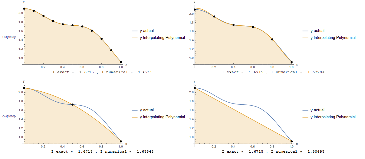
The resulting interpolating polynomials are given by:
![\[\begin{split}y_{h=0.1}&=2.1 + 0.0161419 x - 5.48942 x^2 + 5.32445 x^3 - 6.11881 x^4 + 123.581 x^5 - 356.658 x^6\\& + 389.096 x^7 - 159.091 x^8 - 6.69727 x^9 + 14.8471 x^{10}\\y_{h=0.2}&=2.1 + 1.11382 x - 18.0584 x^2 + 53.5143 x^3 - 61.493 x^4 + 23.7332 x^5\\y_{h=0.5}&=2.1 - 0.298911 x - 0.891185 x^2\\y_{h=1}&=2.1-1.1901x\end{split}\]](https://engcourses-uofa.ca/wp-content/ql-cache/quicklatex.com-2a1a09c1ef3fc047d4cba12bfe01f16b_l3.png "Rendered by QuickLaTeX.com")
Integrating the above formulas is straightforward and the resulting values are:
![\[\begin{split}I_{h=0.1}&=1.6715\\I_{h=0.2}&=1.67294\\I_{h=0.5}&=1.65348\\I_{h=1}&=1.50495\end{split}\]](https://engcourses-uofa.ca/wp-content/ql-cache/quicklatex.com-57fbbba13034acf32d0d50966c54a407_l3.png "Rendered by QuickLaTeX.com")
The following is the Mathematica code used.
View Mathematica Code
h = {0.1, 0.2, 0.5, 1};
n = Table[1/h[[i]] + 1, {i, 1, 4}];
y = 2 - x^2 + 0.1*Cos[2 Pi*x/0.7];
Data = Table[{h[[i]]*(j - 1), (y /. x -> h[[i]]*(j - 1.0))}, {i, 1, 4}, {j, 1, n[[i]]}];
Data // MatrixForm;
p = Table[InterpolatingPolynomial[Data[[i]], x], {i, 1, 4}];
a1 = Plot[{y, p[[1]]}, {x, 0, 1},   Epilog -> {PointSize[Large], Point[Data[[1]]]},   AxesLabel -> {"x", "y"}, BaseStyle -> Bold, ImageSize -> Medium,   PlotRange -> All, Filling -> {2 -> Axis},   PlotLegends -> {"y actual", "y Interpolating Polynomial"}];
a2 = Plot[{y, p[[2]]}, {x, 0, 1},    Epilog -> {PointSize[Large], Point[Data[[2]]]},    AxesLabel -> {"x", "y"}, BaseStyle -> Bold, ImageSize -> Medium,    PlotRange -> All, Filling -> {2 -> Axis},    PlotLegends -> {"y actual", "y Interpolating Polynomial"}];
a3 = Plot[{y, p[[3]]}, {x, 0, 1},    Epilog -> {PointSize[Large], Point[Data[[3]]]},    AxesLabel -> {"x", "y"}, BaseStyle -> Bold, ImageSize -> Medium,    PlotRange -> All, Filling -> {2 -> Axis},    PlotLegends -> {"y actual", "y Interpolating Polynomial"}];
a4 = Plot[{y, p[[4]]}, {x, 0, 1},    Epilog -> {PointSize[Large], Point[Data[[4]]]},    AxesLabel -> {"x", "y"}, BaseStyle -> Bold, ImageSize -> Medium,    PlotRange -> All, Filling -> {2 -> Axis},    PlotLegends -> {"y actual", "y Interpolating Polynomial"}];
Iexact = Integrate[y, {x, 0, 1}];
Inumerical = Table[Integrate[p[[i]], {x, 0, 1}], {i, 1, 4}];
atext = Table[Grid[{{"I exact = ", Iexact, ", I numerical = ", Inumerical[[i]]}}], {i, 1, 4}];
Grid[{{a1, a2}, {atext[[1]], atext[[2]]}}]
Grid[{{a3, a4}, {atext[[3]], atext[[4]]}}]
import numpy as np
import sympy as sp
import matplotlib.pyplot as plt

h = [0.1, 0.2, 0.5, 1]
n = [1/h[i] + 1 for i in range(len(h))]
x = sp.symbols('x')
y = 2 - x**2 + 0.1*sp.cos(2*np.pi*x/0.7)
Data = [[(h[i]*j, (y.subs(x, h[i]*j))) for j in range(int(n[i]))] for i in range(len(h))]
p = [sp.interpolate(Data[i], x) for i in range(len(h))]
x_val = np.arange(0,1,0.01)
Iexact = sp.integrate(y, (x, 0, 1))

plt.xlabel("I exact = "+str(sp.N(Iexact,6)) + " ,   I numerical = "+str(sp.N(sp.integrate(p[0], (x, 0, 1)),6)))
plt.scatter([point[0] for point in Data[0]],[point[1] for point in Data[0]], c='k')
plt.plot(x_val, [y.subs(x,i) for i in x_val], label="y actual")
plt.plot(x_val, [p[0].subs(x,i) for i in x_val], label="y Interpolating Polynomial")
plt.fill_between(x_val, np.float_([p[0].subs(x,i) for i in x_val]), 0, alpha=0.20)
plt.legend(); plt.grid(); plt.show()

plt.xlabel("I exact = "+str(sp.N(Iexact,6)) + " ,   I numerical = "+str(sp.N(sp.integrate(p[1], (x, 0, 1)),6)))
plt.scatter([point[0] for point in Data[1]],[point[1] for point in Data[1]], c='k')
plt.plot(x_val, [y.subs(x,i) for i in x_val], label="y actual")
plt.plot(x_val, [p[1].subs(x,i) for i in x_val], label="y Interpolating Polynomial")
plt.fill_between(x_val, np.float_([p[1].subs(x,i) for i in x_val]), 0, alpha=0.20)
plt.legend(); plt.grid(); plt.show()

plt.xlabel("I exact = "+str(sp.N(Iexact,6)) + " ,   I numerical = "+str(sp.N(sp.integrate(p[2], (x, 0, 1)),6)))
plt.scatter([point[0] for point in Data[2]],[point[1] for point in Data[2]], c='k')
plt.plot(x_val, [y.subs(x,i) for i in x_val], label="y actual")
plt.plot(x_val, [p[2].subs(x,i) for i in x_val], label="y Interpolating Polynomial")
plt.fill_between(x_val, np.float_([p[2].subs(x,i) for i in x_val]), 0, alpha=0.20)
plt.legend(); plt.grid(); plt.show()

plt.xlabel("I exact = "+str(sp.N(Iexact,6)) + " ,   I numerical = "+str(sp.N(sp.integrate(p[3], (x, 0, 1)),6)))
plt.scatter([point[0] for point in Data[3]],[point[1] for point in Data[3]], c='k')
plt.plot(x_val, [y.subs(x,i) for i in x_val], label="y actual")
plt.fill_between(x_val, np.float_([p[3].subs(x,i) for i in x_val]), 0, alpha=0.20)
plt.plot(x_val, [p[3].subs(x,i) for i in x_val], label="y Interpolating Polynomial")
plt.legend(); plt.grid(); plt.show()
The following links provide the MATLAB codes for implementing the integration using the interpolating polynomials
However, as described in the interpolating polynomial section, the larger the degree of the polynomial, the more susceptible it is to oscillations. As an example, the previous problem is repeated with the Runge function defined on the interval from -1 to 1. The figure below shows that using many points leads to large oscillations in the interpolating polynomial which renders the numerical integration largely inaccurate. When fewer points are used, the interpolating polynomial is still highly inaccurate. Therefore, the Newton-Cotes formulas can be applied by simply subdividing the interval into smaller subintervals and applying the Newton-Cotes formulas to each subinterval and adding the results. This process is called: “Composite rules”. The rectangle method, trapezoidal rule, and Simpson’s rules presented in the following sections are specific examples of the composite Newton-Cotes formulas.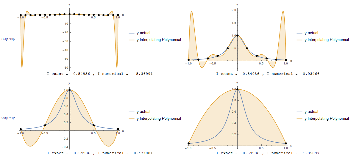
h = {0.1, 0.2, 0.5, 1};
n = Table[2/h[[i]] + 1, {i, 1, 4}];
y = 1.0/(1 + 25 x^2);
Data = Table[{-1 +    h[[i]]*(j - 1), (y /. x -> -1 + h[[i]]*(j - 1.0))}, {i, 1,     4}, {j, 1, n[[i]]}];
Data // MatrixForm;
p = Table[InterpolatingPolynomial[Data[[i]], x], {i, 1, 4}];
a1 = Plot[{y, p[[1]]}, {x, -1, 1},    Epilog -> {PointSize[Large], Point[Data[[1]]]},    AxesLabel -> {"x", "y"}, BaseStyle -> Bold, ImageSize -> Medium,    PlotRange -> All, Filling -> {2 -> Axis},    PlotLegends -> {"y actual", "y Interpolating Polynomial"}];
a2 = Plot[{y, p[[2]]}, {x, -1, 1},    Epilog -> {PointSize[Large], Point[Data[[2]]]},    AxesLabel -> {"x", "y"}, BaseStyle -> Bold, ImageSize -> Medium,    PlotRange -> All, Filling -> {2 -> Axis},    PlotLegends -> {"y actual", "y Interpolating Polynomial"}];
a3 = Plot[{y, p[[3]]}, {x, -1, 1},    Epilog -> {PointSize[Large], Point[Data[[3]]]},    AxesLabel -> {"x", "y"}, BaseStyle -> Bold, ImageSize -> Medium,    PlotRange -> All, Filling -> {2 -> Axis},    PlotLegends -> {"y actual", "y Interpolating Polynomial"}];
a4 = Plot[{y, p[[4]]}, {x, -1, 1},    Epilog -> {PointSize[Large], Point[Data[[4]]]},    AxesLabel -> {"x", "y"}, BaseStyle -> Bold, ImageSize -> Medium,    PlotRange -> All, Filling -> {2 -> Axis},    PlotLegends -> {"y actual", "y Interpolating Polynomial"}];
Iexact = Integrate[y, {x, -1, 1}];
Inumerical = Table[Integrate[p[[i]], {x, -1, 1}], {i, 1, 4}];

atext = Table[   Grid[{{"I exact = ", Iexact, ", I numerical = ",  Inumerical[[i]]}}], {i, 1, 4}];
Grid[{{a1, a2}, {atext[[1]], atext[[2]]}}]
Grid[{{a3, a4}, {atext[[3]], atext[[4]]}}]
import numpy as np
import sympy as sp
import matplotlib.pyplot as plt

h = [0.1, 0.2, 0.5, 1]
n = [2/h[i] + 1 for i in range(len(h))]
x = sp.symbols('x')
y = 1.0/(1 + 25*x**2)
Data = [[(-1 + h[i]*j, (y.subs(x, -1 + h[i]*j))) for j in range(int(n[i]))] for i in range(len(h))]
p = [sp.interpolate(Data[i], x) for i in range(len(h))]
x_val = np.arange(-1,1,0.01)
Iexact = sp.integrate(y, (x, -sp.oo, sp.oo))

plt.xlabel("I exact = "+str(sp.N(Iexact,6)) + " ,   I numerical = "+str(sp.N(sp.integrate(p[0], (x, -1, 1)),6)))
plt.scatter([point[0] for point in Data[0]],[point[1] for point in Data[0]], c='k')
plt.plot(x_val, [y.subs(x,i) for i in x_val], label="y actual")
plt.plot(x_val, [p[0].subs(x,i) for i in x_val], label="y Interpolating Polynomial")
plt.fill_between(x_val, np.float_([p[0].subs(x,i) for i in x_val]), 0, alpha=0.20)
plt.legend(); plt.grid(); plt.show()

plt.xlabel("I exact = "+str(sp.N(Iexact,6)) + " ,   I numerical = "+str(sp.N(sp.integrate(p[1], (x, -1, 1)),6)))
plt.scatter([point[0] for point in Data[1]],[point[1] for point in Data[1]], c='k')
plt.plot(x_val, [y.subs(x,i) for i in x_val], label="y actual")
plt.plot(x_val, [p[1].subs(x,i) for i in x_val], label="y Interpolating Polynomial")
plt.fill_between(x_val, np.float_([p[1].subs(x,i) for i in x_val]), 0, alpha=0.20)
plt.legend(); plt.grid(); plt.show()

plt.xlabel("I exact = "+str(sp.N(Iexact,6)) + " ,   I numerical = "+str(sp.N(sp.integrate(p[2], (x, -1, 1)),6)))
plt.scatter([point[0] for point in Data[2]],[point[1] for point in Data[2]], c='k')
plt.plot(x_val, [y.subs(x,i) for i in x_val], label="y actual")
plt.plot(x_val, [p[2].subs(x,i) for i in x_val], label="y Interpolating Polynomial")
plt.fill_between(x_val, np.float_([p[2].subs(x,i) for i in x_val]), 0, alpha=0.20)
plt.legend(); plt.grid(); plt.show()

plt.xlabel("I exact = "+str(sp.N(Iexact,6)) + " ,   I numerical = "+str(sp.N(sp.integrate(p[3], (x, -1, 1)),6)))
plt.scatter([point[0] for point in Data[3]],[point[1] for point in Data[3]], c='k')
plt.plot(x_val, [y.subs(x,i) for i in x_val], label="y actual")
plt.fill_between(x_val, np.float_([p[3].subs(x,i) for i in x_val]), 0, alpha=0.20)
plt.plot(x_val, [p[3].subs(x,i) for i in x_val], label="y Interpolating Polynomial")
plt.legend(); plt.grid(); plt.show()
The following tool which appears on MecsimCalc provides a visual representation of different numerical integration schemes that are studied in later sections: