
Nonlinear Systems of Equations: Newton-Raphson Method
Newton-Raphson Method
The Newton-Raphson method is the method of choice for solving nonlinear systems of equations. Many engineering software packages (especially finite element analysis software) that solve nonlinear systems of equations use the Newton-Raphson method. The derivation of the method for nonlinear systems is very similar to the one-dimensional version in the root finding section. Assume a nonlinear system of equations of the form:
![\[\begin{split} f_1(x_1,x_2,\cdots,x_n)&=0\\ f_2(x_1,x_2,\cdots,x_n)&=0\\ &\vdots\\ f_n(x_1,x_2,\cdots,x_n)&=0 \end{split} \]](https://engcourses-uofa.ca/wp-content/ql-cache/quicklatex.com-09564db9f5b122a6ef7dd81f8b73e427_l3.png "Rendered by QuickLaTeX.com")
If the components of one iteration  are known as:
  , then, the Taylor expansion of the first equation around these components is given by:
![\[\begin{split} f_1\left(x_1^{(i+1)},x_2^{(i+1)},\cdots,x_n^{(i+1)}\right)\approx&f_1\left(x_1^{(i)},x_2^{(i)},\cdots,x_n^{(i)}\right)+\\ &\frac{\partial f_1}{\partial x_1}\bigg|_{x^{(i)}}\left(x_1^{(i+1)}-x_1^{(i)}\right)+\frac{\partial f_1}{\partial x_2}\bigg|_{x^{(i)}}\left(x_2^{(i+1)}-x_2^{(i)}\right)+\cdots+\\ &\frac{\partial f_1}{\partial x_n}\bigg|_{x^{(i)}}\left(x_n^{(i+1)}-x_n^{(i)}\right) \end{split} \]](https://engcourses-uofa.ca/wp-content/ql-cache/quicklatex.com-f24fbf8fb01b29027ce0d4a3e952a9c1_l3.png "Rendered by QuickLaTeX.com")
Applying the Taylor expansion in the same manner for  , we obtained the following system of linear equations with the unknowns being the components of the vector
  :
:
![\[ \left(\begin{array}{c}f_1\left(x^{(i+1)}\right)\\f_2\left(x^{(i+1)}\right)\\\vdots \\ f_n\left(x^{(i+1)}\right)\end{array}\right) = \left(\begin{array}{c}f_1\left(x^{(i)}\right)\\f_2\left(x^{(i)}\right)\\\vdots \\ f_n\left(x^{(i)}\right)\end{array}\right)+ \left(\begin{matrix}\frac{\partial f_1}{\partial x_1}\big|_{x^{(i)}} & \frac{\partial f_1}{\partial x_2}\big|_{x^{(i)}} &\cdots&\frac{\partial f_1}{\partial x_n}\big|_{x^{(i)}} \\\frac{\partial f_2}{\partial x_1}\big|_{x^{(i)}} & \frac{\partial f_2}{\partial x_2}\big|_{x^{(i)}} & \cdots & \frac{\partial f_2}{\partial x_n}\big|_{x^{(i)}}\\\vdots&\vdots&\vdots&\vdots\\ \frac{\partial f_n}{\partial x_1}\big|_{x^{(i)}} & \frac{\partial f_n}{\partial x_2}\big|_{x^{(i)}} &\cdots& \frac{\partial f_n}{\partial x_n}\big|_{x^{(i)}} \end{matrix}\right)\left(\begin{array}{c}\left(x_1^{(i+1)}-x_1^{(i)}\right)\\\left(x_2^{(i+1)}-x_2^{(i)}\right)\\\vdots\\\left(x_n^{(i+1)}-x_n^{(i)}\right)\end{array}\right) \]](https://engcourses-uofa.ca/wp-content/ql-cache/quicklatex.com-3d7617d7ec3b6f0025bc5d7ff75ea76d_l3.png "Rendered by QuickLaTeX.com")
By setting the left hand side to zero (which is the desired value for the functions  , then, the system can be written as:
![\[ \left(\begin{matrix}\frac{\partial f_1}{\partial x_1}\big|_{x^{(i)}} & \frac{\partial f_1}{\partial x_2}\big|_{x^{(i)}} &\cdots&\frac{\partial f_1}{\partial x_n}\big|_{x^{(i)}} \\\frac{\partial f_2}{\partial x_1}\big|_{x^{(i)}} & \frac{\partial f_2}{\partial x_2}\big|_{x^{(i)}} & \cdots & \frac{\partial f_2}{\partial x_n}\big|_{x^{(i)}}\\\vdots&\vdots&\vdots&\vdots\\ \frac{\partial f_n}{\partial x_1}\big|_{x^{(i)}} & \frac{\partial f_n}{\partial x_2}\big|_{x^{(i)}} &\cdots& \frac{\partial f_n}{\partial x_n}\big|_{x^{(i)}} \end{matrix}\right)\left(\begin{array}{c}\left(x_1^{(i+1)}-x_1^{(i)}\right)\\\left(x_2^{(i+1)}-x_2^{(i)}\right)\\\vdots\\\left(x_n^{(i+1)}-x_n^{(i)}\right)\end{array}\right)= -\left(\begin{array}{c}f_1\left(x^{(i)}\right)\\f_2\left(x^{(i)}\right)\\\vdots \\ f_n\left(x^{(i)}\right)\end{array}\right) \]](https://engcourses-uofa.ca/wp-content/ql-cache/quicklatex.com-638c516ce27af32edb0bd2968e6d8776_l3.png "Rendered by QuickLaTeX.com")
Setting  , the above equation can be written in matrix form as follows:
![\[ K \Delta x=-f \]](https://engcourses-uofa.ca/wp-content/ql-cache/quicklatex.com-95d779e4ff0bf3641210daa38432f540_l3.png "Rendered by QuickLaTeX.com")
where  is an
is an  matrix,
  is a vector of
  components and
  is an -dimensional vector with the components
  . If is invertible, then, the above system can be solved as follows:
![\[ \Delta x = -K^{-1}f \Rightarrow x^{(i+1)}=x^{(i)}+\Delta x \]](https://engcourses-uofa.ca/wp-content/ql-cache/quicklatex.com-4ec7771d6f991a10b9f9be1e8ed84590_l3.png "Rendered by QuickLaTeX.com")
Example
Use the Newton-Raphson method with  to find the solution to the following nonlinear system of equations:
![\[ x_1^2+x_1x_2=10\qquad x_2+3x_1x_2^2=57 \]](https://engcourses-uofa.ca/wp-content/ql-cache/quicklatex.com-629a2dce646e445532afcc293024d850_l3.png "Rendered by QuickLaTeX.com")
Solution
In addition to requiring an initial guess, the Newton-Raphson method requires evaluating the derivatives of the functions  and
and  . If
. If  , then it has the following form:
![\[ K=\left(\begin{matrix}\frac{\partial f_1}{\partial x_1}& \frac{\partial f_1}{\partial x_2}\\\frac{\partial f_2}{\partial x_1} & \frac{\partial f_2}{\partial x_2}\end{matrix}\right)=\left(\begin{matrix}2x_1+x_2& x_1\\3x_2^2 & 1+6x_1x_2\end{matrix}\right) \]](https://engcourses-uofa.ca/wp-content/ql-cache/quicklatex.com-3891cede2c9a5c70cb97cfeb19cefe9f_l3.png "Rendered by QuickLaTeX.com")
Assuming an initial guess of  and
and  , then the vector
  and the matrix have components:
![\[ f=\left(\begin{array}{c}x_1^2+x_1x_2-10\\x_2+3x_1x_2^2-57\end{array}\right)=\left(\begin{array}{c}-2.5\\1.625\end{array}\right) \qquad K=\left(\begin{matrix}6.5 & 1.5 \\ 36.75 & 32.5\end{matrix}\right) \]](https://engcourses-uofa.ca/wp-content/ql-cache/quicklatex.com-ab2be4d937a949e0892e6cbe4cda5577_l3.png "Rendered by QuickLaTeX.com")
The components of the vector can be computed as follows:
![\[ \Delta x = -K^{-1}f=\left(\begin{array}{c}0.53603\\-0.65612\end{array}\right) \]](https://engcourses-uofa.ca/wp-content/ql-cache/quicklatex.com-9b4123c2277ba8499113670d360bb1c6_l3.png "Rendered by QuickLaTeX.com")
Therefore, the new estimates for  and
and  are:
are:
![\[ x^{(1)}=x^{(0)}+\Delta x=\left(\begin{array}{c}2.036029\\2.843875\end{array}\right) \]](https://engcourses-uofa.ca/wp-content/ql-cache/quicklatex.com-bed4bee695d89da186e39399a3267ec2_l3.png "Rendered by QuickLaTeX.com")
The approximate relative error is given by:
![\[ \varepsilon_r=\frac{\sqrt{(0.53603)^2+(-0.65612)^2}}{\sqrt{(2.036029)^2+(2.843875)^2}}=0.2422 \]](https://engcourses-uofa.ca/wp-content/ql-cache/quicklatex.com-390ce03c03a29d0aedaef41555c10b1f_l3.png "Rendered by QuickLaTeX.com")
For the second iteration the vector and the matrix have components:
![\[ f=\left(\begin{array}{c}-0.06437\\-4.75621\end{array}\right) \qquad K=\left(\begin{matrix}6.9159 & 2.0360 \\ 24.2629 & 35.7413\end{matrix}\right) \]](https://engcourses-uofa.ca/wp-content/ql-cache/quicklatex.com-508063a6504d7a676306f2dbda24f0fa_l3.png "Rendered by QuickLaTeX.com")
The components of the vector can be computed as follows:
![\[ \Delta x = -K^{-1}f=\left(\begin{array}{c}-0.03733\\0.15841\end{array}\right) \]](https://engcourses-uofa.ca/wp-content/ql-cache/quicklatex.com-d91be0f80a8d5e6038c48a61e2169ee1_l3.png "Rendered by QuickLaTeX.com")
Therefore, the new estimates for  and
and  are:
are:
![\[ x^{(2)}=x^{(1)}+\Delta x=\left(\begin{array}{c}1.998701\\3.002289\end{array}\right) \]](https://engcourses-uofa.ca/wp-content/ql-cache/quicklatex.com-ecc9e0c28e5c561187743ac03f6bb70d_l3.png "Rendered by QuickLaTeX.com")
The approximate relative error is given by:
![\[ \varepsilon_r=\frac{\sqrt{(-0.03733)^2+(0.15841)^2}}{\sqrt{(1.998701)^2+(3.002289)^2}}=0.04512 \]](https://engcourses-uofa.ca/wp-content/ql-cache/quicklatex.com-d9385063946dbfd07c37abedc1a266d6_l3.png "Rendered by QuickLaTeX.com")
For the third iteration the vector and the matrix have components:
![\[ f=\left(\begin{array}{c}-0.00452\\0.04957\end{array}\right) \qquad K=\left(\begin{matrix}6.9997 & 1.9987 \\ 27.0412 & 37.0041\end{matrix}\right) \]](https://engcourses-uofa.ca/wp-content/ql-cache/quicklatex.com-71899249329b64cf887bbe02230d93a5_l3.png "Rendered by QuickLaTeX.com")
The components of the vector can be computed as follows:
![\[ \Delta x = -K^{-1}f=\left(\begin{array}{c}0.00130\\-0.00229\end{array}\right) \]](https://engcourses-uofa.ca/wp-content/ql-cache/quicklatex.com-c6547342d1cffa3e8985c49e5f43c039_l3.png "Rendered by QuickLaTeX.com")
Therefore, the new estimates for  and
and  are:
are:
![\[ x^{(3)}=x^{(2)}+\Delta x=\left(\begin{array}{c}2.00000\\2.999999\end{array}\right) \]](https://engcourses-uofa.ca/wp-content/ql-cache/quicklatex.com-4349b1b31af5408e2bab3cb6f4749af5_l3.png "Rendered by QuickLaTeX.com")
The approximate relative error is given by:
![\[ \varepsilon_r=\frac{\sqrt{(0.00130)^2+(-0.00229)^2}}{\sqrt{(2.00000)^2+(2.999999)^2}}=0.00073 \]](https://engcourses-uofa.ca/wp-content/ql-cache/quicklatex.com-541629c0ed37f16c4446aef7c87e8314_l3.png "Rendered by QuickLaTeX.com")
Finally, for the fourth iteration the vector and the matrix have components:
![\[ f=\left(\begin{array}{c}0.00000\\-0.00002\end{array}\right) \qquad K=\left(\begin{matrix}7 & 2 \\ 27 & 37\end{matrix}\right) \]](https://engcourses-uofa.ca/wp-content/ql-cache/quicklatex.com-e3d72430b60ddac4d4d8ea432f7a75fd_l3.png "Rendered by QuickLaTeX.com")
The components of the vector can be computed as follows:
![\[ \Delta x = -K^{-1}f=\left(\begin{array}{c}0.00000\\0.00000\end{array}\right) \]](https://engcourses-uofa.ca/wp-content/ql-cache/quicklatex.com-5e1fbec24221643bd02754320778d23b_l3.png "Rendered by QuickLaTeX.com")
Therefore, the new estimates for  and
and  are:
are:
![\[ x^{(4)}=x^{(3)}+\Delta x=\left(\begin{array}{c}2\\3\end{array}\right) \]](https://engcourses-uofa.ca/wp-content/ql-cache/quicklatex.com-be9ffdb6b2a3cf39d6df96c3e36175e2_l3.png "Rendered by QuickLaTeX.com")
The approximate relative error is given by:
![\[ \varepsilon_r=\frac{\sqrt{(0.00000)^2+(0.00000)^2}}{\sqrt{(2)^2+(3)^2}}=0.00000 \]](https://engcourses-uofa.ca/wp-content/ql-cache/quicklatex.com-db691cf8afd98635fdb38aeb24e6d676_l3.png "Rendered by QuickLaTeX.com")
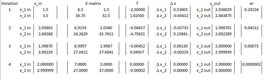
Therefore, convergence is achieved after 4 iterations which is much faster than the 9 iterations in the fixed-point iteration method. The following is the Microsoft Excel table showing the values generated in every iteration:
The Newton-Raphson method can be implemented directly in Mathematica using the “FindRoot” built-in function:
View Mathematica CodeFindRoot[{x1^2 + x1*x2 - 10 == 0, x2 + 3*x1*x2^2 == 57}, {{x1, 1.5}, {x2, 3.5}}]
# Using Sympy
import sympy as sp
x1, x2 = sp.symbols('x1 x2')
sol = sp.nsolve((x1**2 + x1*x2 - 10, x2 + 3*x1*x2**2 - 57), (x1,x2), (1.5,3.5))
print("Sympy: ",sol)

# Using Scipy's root
from scipy.optimize import root
def equations(x):
  x1, x2 = x
  return [x1**2 + x1*x2 - 10,
          x2 + 3*x1*x2**2 - 57]
sol = root(equations, [1.5,3.5])
print("Scipy: ",sol.x)
MATLAB code for the Newton-Raphson example
MATLAB file 1 (nrsystem.m)
MATLAB file 2 (f.m)
MATLAB file 3 (K.m)
The following “While” loop in Mathematica provides an iterative procedure that implements the Newton-Raphson Method in Mathematica and produces the table shown:
View Mathematica Codex = {x1, x2};
f1 = x1^2 + x1*x2 - 10;
f2 = x2 + 3 x1*x2^2 - 57;
f = {f1, f2};
K = Table[D[f[[i]], x[[j]]], {i, 1, 2}, {j, 1, 2}];
K // MatrixForm
xtable = {{1.5, 3.5}};
xrule = {{x1 -> xtable[[1, 1]], x2 -> xtable[[1, 2]]}};
Ertable = {1}
NMax = 100;
i = 1;
eps = 0.000001
While[And[Ertable[[i]] > eps, i <= NMax],
Delta = -(Inverse[K].f) /. xrule[[i]];
xtable = Append[xtable, Delta + xtable[[Length[xtable]]]];
xrule = Append[
xrule, {x1 -> xtable[[Length[xtable], 1]],
x2 -> xtable[[Length[xtable], 2]]}];
er = Norm[Delta]/Norm[xtable[[i+1]]]; Ertable = Append[Ertable, er]; i++]
Title = {"Iteration", "x1_in", "x2_in", "x1_out", "x2_out", "er"};
T2 = Table[{i, xtable[[i, 1]], xtable[[i, 2]], xtable[[i + 1, 1]], xtable[[i + 1, 2]], Ertable[[i + 1]]}, {i, 1, Length[xtable] - 1}];
T2 = Prepend[T2, Title];
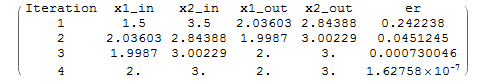
T2 // MatrixForm
import numpy as np
import sympy as sp
import pandas as pd

x1, x2 = sp.symbols('x1 x2')
x = [x1, x2]
f1 = x1**2 + x1*x2 - 10
f2 = x2 + 3*x1*x2**2 - 57
f = sp.Matrix([f1, f2])
K = sp.Matrix([[f[i].diff(x[j]) for j in range(2)] for i in range(2)])
xtable = [[1.5, 3.5]]
Ertable = [1]
NMax = 100
i = 0
eps = 0.000001
Delta = -(K.inv()*f)

while Ertable[i] > eps and i <= NMax:
  xtable.append(np.add(list(Delta.subs({x1:xtable[-1][0], x2:xtable[-1][1]})), xtable[-1]))
  er = np.linalg.norm(np.array(Delta.subs({x1:xtable[-2][0], x2:xtable[-2][1]})).astype(np.float64))/np.linalg.norm(np.array(xtable[i+1]).astype(np.float64))
  Ertable.append(er)
  i+=1

T2 = [[i + 1, xtable[i][0], xtable[i][1], xtable[i + 1][0], xtable[i + 1][1], Ertable[i + 1]] for i in range(len(xtable) - 1)]
T2 = pd.DataFrame(T2, columns=["Iteration", "x1_in", "x2_in", "x1_out", "x2_out", "er"])
display(T2)
Thank you Dr. Samer and Dr. Linsey and the entire team, for a great and very informative lectures notes, educational videos.
My best and sincere regards… Naim
Thank you very much for these good notes. Kindly send me the pdf of the entire notes if possible. Be blessed
Can we solve n equations with n unknowns using this method?
Is there any Mathematica code to solve system of n equations with n unknowns? Let us know.
numerical analysis
Kindly send me the pdf version of your notes. I will appreciate it. Thanking you for work