
Solution Methods for IVPs: Backward (Implicit) Euler Method
Backward (Implicit) Euler Method
Consider the following IVP:
![\[\frac{\mathrm{d}x}{\mathrm{d}t}=F(x,t)\]](https://engcourses-uofa.ca/wp-content/ql-cache/quicklatex.com-6ed9b113848557dfe067ea60ab3c48c9_l3.png "Rendered by QuickLaTeX.com")
Assuming that the value of the dependent variable  (say
(say  ) is known at an initial value
  , then, we can use a Taylor approximation to relate the value of at
  , namely
  with
with  . However, unlike the explicit Euler method, we will use the Taylor series around the point , that is:
![\[x_i=x(t_{i+1})-\frac{\mathrm{d}x}{\mathrm{d}t}\bigg|_{t_{i+1}} (h) +\mathcal{O}(h^2)\]](https://engcourses-uofa.ca/wp-content/ql-cache/quicklatex.com-da10c848f27f2f0d6be39b341dd2d486_l3.png "Rendered by QuickLaTeX.com")
Substituting the differential equation into the above equation yields:
![\[x_i=x(t_{i+1})-F(x_{i+1},t_{i+1}) (h) +\mathcal{O}(h^2)\]](https://engcourses-uofa.ca/wp-content/ql-cache/quicklatex.com-feac6e7cc6b2f532513ac9fe69251de7_l3.png "Rendered by QuickLaTeX.com")
Therefore, as an approximation, an estimate for can be taken as  as follows:
![\[x(t_{i+1})\approx x_{i+1}=x_i+F(x_{i+1},t_{i+1}) (h)\]](https://engcourses-uofa.ca/wp-content/ql-cache/quicklatex.com-b4c2790ccbbd9c8fb9b384a769c08166_l3.png "Rendered by QuickLaTeX.com")
Using this estimate, the local truncation error is thus proportional to the square of the step size with the constant of proportionality related to the second derivative of , which is the first derivative of the given IVP. The backward Euler method is termed an “implicit” method because it uses the slope  at the unknown point , namely:
  . The developed equation can be linear in or nonlinear. Nonlinear equations can often be solved using the fixed-point iteration method or the Newton-Raphson method to find the value of . While the implicit scheme does not provide better accuracy than the explicit scheme, it comes with additional computations. However, one advantage is that this scheme is always stable.
The following Mathematica code adopts the implicit Euler scheme and uses the built-in FindRoot function to solve for . The code is similar to the code provided for the explicit scheme except for the line to calculate .
ImplicitEulerMethod[fp_, x0_, h_, t0_, tmax_] :=
(n = (tmax - t0)/h + 1;
 xtable = Table[0, {i, 1, n}];
 xtable[[1]] = x0;
 Do[  s = FindRoot[x == xtable[[i - 1]] + h*fp[x, t0 + (i - 1) h], {x, xtable[[i - 1]]}];  xtable[[i]] = x /. s[[1]],  {i, 2, n}];
  Data = Table[{t0 + (i - 1)*h, xtable[[i]]}, {i, 1, n}];
  Data)

function1[y_, t_] := 0.05 y
function2[x_, t_] := 0.015 x
ImplicitEulerMethod[function1, 35, 1.0, 0, 50] // MatrixForm
ImplicitEulerMethod[function2, 35, 1.0, 0, 50] // MatrixForm
import numpy as np
import sympy as sp
x = sp.symbols('x')
def ImplicitEulerMethod(fp, x0, h, t0, tmax):
  n = int((tmax - t0)/h + 1)
  xtable = [0 for i in range(n)]
  xtable[0] = x0
  for i in range(1,n):
    s = sp.nsolve(x - xtable[i - 1] - h*fp(x, t0 + i*h), x, xtable[i - 1])
    xtable[i] = s
  Data = [[t0 + i*h, xtable[i]] for i in range(n)]
  return Data

def function1(y, t): return 0.05*y
def function2(x, t): return 0.015*x
print(np.vstack(ImplicitEulerMethod(function1, 35, 1.0, 0, 50)))
print(np.vstack(ImplicitEulerMethod(function2, 35, 1.0, 0, 50)))
Example 1
Repeat Example 1 above using the implicit Euler method.
Solution
When  , the IVP is given by:
![\[\frac{\mathrm{d}x}{\mathrm{d}t}=0.015 x\]](https://engcourses-uofa.ca/wp-content/ql-cache/quicklatex.com-5da4656634a270c31768984ebd63089b_l3.png "Rendered by QuickLaTeX.com")
Given a value for at , and taking  , the estimate for can be calculated according to the formula:
![\[x_{i+1}=x_i+h\frac{\mathrm{d}x}{\mathrm{d}t}\bigg|_{x=x_{i+1},t=t_{i+1}}=x_i+h(0.015x_{i+1})\]](https://engcourses-uofa.ca/wp-content/ql-cache/quicklatex.com-08d3b15bf5aca1f37756beb9ff93c2f9_l3.png "Rendered by QuickLaTeX.com")
Rearranging yields:
![\[x_{i+1}=\frac{x_i}{1-0.015}\]](https://engcourses-uofa.ca/wp-content/ql-cache/quicklatex.com-4708976158f9e7fba2539b16a62cec55_l3.png "Rendered by QuickLaTeX.com")
With  million and
  years, the estimate for the population at
  years using the implicit Euler method is given by:
![\[x_1=\frac{35}{1-0.015}=35.533\]](https://engcourses-uofa.ca/wp-content/ql-cache/quicklatex.com-3a47ceed0a506c2c380f8b40569bb60d_l3.png "Rendered by QuickLaTeX.com")
at  years, the value of
  in millions is given by:
![\[x_2=\frac{35.533}{1-0.015}=36.074\]](https://engcourses-uofa.ca/wp-content/ql-cache/quicklatex.com-d84fbabcb197ecaaec689effd9ce7c98_l3.png "Rendered by QuickLaTeX.com")
Proceeding iteratively, the following is the Excel table showing the values of the population up to  years.
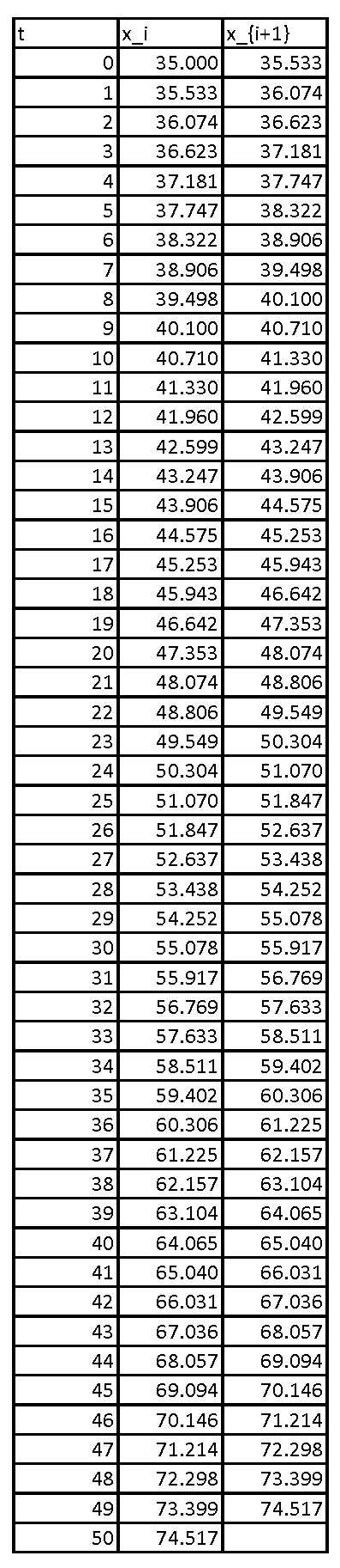
When , the implicit method provides an error similar to that of the explicit method:
![\[\begin{split}E&=35e^{(0.015\times 50)}-74.517=74.095-74.517=-0.4\\E_r&=\frac{-0.4}{74.095}=-0.005\end{split}\]](https://engcourses-uofa.ca/wp-content/ql-cache/quicklatex.com-f0b733de9c52ab9b9acb05d7cca0c663_l3.png "Rendered by QuickLaTeX.com")
When  , the IVP is given by:
![\[\frac{\mathrm{d}x}{\mathrm{d}t}=0.05 x\]](https://engcourses-uofa.ca/wp-content/ql-cache/quicklatex.com-472da13c341b10ee92352d29470bec24_l3.png "Rendered by QuickLaTeX.com")
Given a value for at , and taking , the estimate for can be calculated according to the formula:
![\[x_{i+1}=x_i+h\frac{\mathrm{d}x}{\mathrm{d}t}\bigg|_{x=x_{i+1},t=t_{i+1}}=x_i+h(0.05x_{i+1})\]](https://engcourses-uofa.ca/wp-content/ql-cache/quicklatex.com-a75d964b12611a94636436e26f5f6767_l3.png "Rendered by QuickLaTeX.com")
Rearranging yields:
![\[x_{i+1}=\frac{x_i}{1-0.05}\]](https://engcourses-uofa.ca/wp-content/ql-cache/quicklatex.com-5a5944801e818897aec612c0b07c3bb9_l3.png "Rendered by QuickLaTeX.com")
With million and years, the estimate for the population at years using the implicit Euler method is given by:
![\[x_1=\frac{35}{1-0.05}=36.842\]](https://engcourses-uofa.ca/wp-content/ql-cache/quicklatex.com-8ad30fe8ef61d226de39f56530715a37_l3.png "Rendered by QuickLaTeX.com")
at years, the value of in millions is given by:
![\[x_2=\frac{36.842}{1-0.05}=38.781\]](https://engcourses-uofa.ca/wp-content/ql-cache/quicklatex.com-83159c0b243ef84c823e2ff85fb127ec_l3.png "Rendered by QuickLaTeX.com")
Proceeding iteratively, the following is the Excel table showing the values of the population up to years.
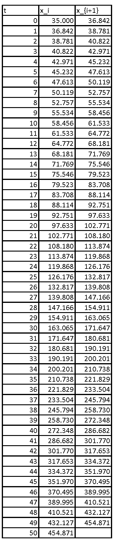
Again, the error produced by the implicit method is comparable to that produced by the explicit method shown above:
![\[\begin{split}E&=35e^{(0.05\times 50)}-454.871=426.387-454.871=-28.483\\E_r&=\frac{-28.483}{426.387}=-0.07\end{split}\]](https://engcourses-uofa.ca/wp-content/ql-cache/quicklatex.com-184f0f699f2007d0cfcc2e8db299a035_l3.png "Rendered by QuickLaTeX.com")
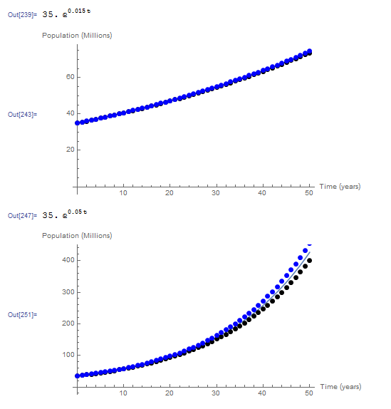
The following is the graph showing the exact solution versus the data using both the implicit (blue dots) and the explicit (black dots) Euler method for both values of  .
.
View Mathematica Code
EulerMethod[fp_, x0_, h_, t0_, tmax_] :=
(n = (tmax - t0)/h + 1;
  xtable = Table[0, {i, 1, n}];
  xtable[[1]] = x0;
  Do[xtable[[i]] = xtable[[i - 1]] + h*fp[xtable[[i - 1]], t0 + (i - 2) h], {i, 2, n}];
  Data = Table[{t0 + (i - 1)*h, xtable[[i]]}, {i, 1, n}];
  Data)

ImplicitEulerMethod[fp_, x0_, h_, t0_,  tmax_] :=
(n = (tmax - t0)/h + 1;
  xtable = Table[0, {i, 1, n}];
  xtable[[1]] = x0;
  Do[s = FindRoot[x == xtable[[i - 1]] + h*fp[x, t0 + (i - 1) h], {x, xtable[[i - 1]]}]; xtable[[i]] = x /. s[[1]], {i, 2, n}];
  Data2 = Table[{t0 + (i - 1)*h, xtable[[i]]}, {i, 1, n}];
  Data2)

Clear[x, xtable]
k = 0.015;
a = DSolve[{x'[t] == k*x[t], x[0] == 35}, x, t];
x = x[t] /. a[[1]]
fp[x_, t_] := k*x;
Data = EulerMethod[fp, 35, 1.0, 0, 50];
Data2 = ImplicitEulerMethod[fp, 35, 1.0, 0, 50];
Plot[x, {t, 0, 50}, Epilog -> {PointSize[Large], Point[Data], Blue, Point[Data2]}, AxesOrigin -> {0, 0}, AxesLabel -> {"Time (years)", "Population (Millions)"}]

Clear[x, xtable]
k = 0.05;
a = DSolve[{x'[t] == k*x[t], x[0] == 35}, x, t];
x = x[t] /. a[[1]]
fp[x_, t_] := k*x;
Data = EulerMethod[fp, 35, 1.0, 0, 50];
Data2 = ImplicitEulerMethod[fp, 35, 1.0, 0, 50];
Plot[x, {t, 0, 50}, Epilog -> {PointSize[Large], Point[Data], Blue, Point[Data2]}, AxesOrigin -> {0, 0}, AxesLabel -> {"Time (years)", "Population (Millions)"}]
# UPGRADE: need Sympy 1.2 or later, upgrade by running: "!pip install sympy --upgrade" in a code cell
# !pip install sympy --upgrade
import numpy as np
import sympy as sp
import matplotlib.pyplot as plt
sp.init_printing(use_latex=True)

def EulerMethod(fp, x0, h, t0, tmax):
  n = int((tmax - t0)/h + 1)
  xtable = [0 for i in range(n)]
  xtable[0] = x0
  for i in range(1,n):
    xtable[i] = xtable[i - 1] + h*fp(xtable[i - 1], t0 + (i - 1)*h)
  Data = [[t0 + i*h, xtable[i]] for i in range(n)]
  return Data

def ImplicitEulerMethod(fp, x0, h, t0, tmax):
  n = int((tmax - t0)/h + 1)
  xtable = [0 for i in range(n)]
  xtable[0] = x0
  x = sp.symbols('x')
  for i in range(1,n):
    s = sp.nsolve(x - xtable[i - 1] - h*fp(x, t0 + i*h), x, xtable[i - 1])
    xtable[i] = s
  Data = [[t0 + i*h, xtable[i]] for i in range(n)]
  return Data

x = sp.Function('x')
t = sp.symbols('t')
k = 0.015
sol = sp.dsolve(x(t).diff(t) - k*x(t), ics={x(0): 35})
display(sol)
def fp(x, t): return k*x
Data = EulerMethod(fp, 35, 1.0, 0, 50)
Data2 = ImplicitEulerMethod(fp, 35, 1.0, 0, 50)
x_val = np.arange(0,50,0.1)
plt.plot(x_val, [sol.subs(t, i).rhs for i in x_val])
plt.scatter([point[0] for point in Data],[point[1] for point in Data])
plt.scatter([point[0] for point in Data2],[point[1] for point in Data2])
plt.xlabel("Time (years)"); plt.ylabel("Population (Millions)")
plt.grid(); plt.show()

k = 0.05
sol = sp.dsolve(x(t).diff(t) - k*x(t), ics={x(0): 35})
display(sol)
Data = EulerMethod(fp, 35, 1.0, 0, 50)
Data2 = ImplicitEulerMethod(fp, 35, 1.0, 0, 50)
plt.plot(x_val, [sol.subs(t, i).rhs for i in x_val])
plt.scatter([point[0] for point in Data],[point[1] for point in Data])
plt.scatter([point[0] for point in Data2],[point[1] for point in Data2])
plt.xlabel("Time (years)"); plt.ylabel("Population (Millions)")
plt.grid(); plt.show()
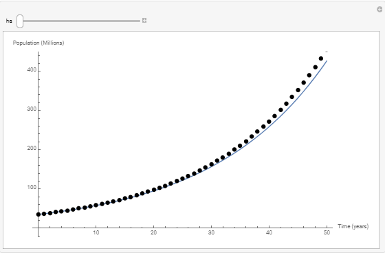
The following tool illustrates the effect of choosing the step size  on the difference between the numerical solution obtained using the implicit methods (shown as dots) and the exact solution (shown as the blue curve) for the case when . The smaller the step size, the more accurate the solution is. The higher the value of , the more the numerical solution deviates from the exact solution. The error increases away from the initial conditions.
Example 2
Repeat Example 2 above using the implicit Euler method.
Solution
Recall that the IVP for this problem is given by:
![\[\frac{\mathrm{d}c}{\mathrm{d}t}=\frac{\left(100+50\cos{(2\pi t/365)}\right)}{10000}\left(5e^{\left(\frac{-2t}{1000}\right)}-c\right)\]](https://engcourses-uofa.ca/wp-content/ql-cache/quicklatex.com-5b02bdc118fd5c27ea1568ff957771ba_l3.png "Rendered by QuickLaTeX.com")
Taking  day,
day,  can be predicted for a given value of
  using the implicit Euler method as follows:
![\[c_{i+1}=c_i+h\frac{\mathrm{d}c}{\mathrm{d}t}\bigg|_{c=c_{i+1},t=t_{i+1}}=c_i+\frac{\left(100+50\cos{(2\pi t_{i+1}/365)}\right)}{10000}\left(5e^{\left(\frac{-2t_{i+1}}{1000}\right)}-c_{i+1}\right)\]](https://engcourses-uofa.ca/wp-content/ql-cache/quicklatex.com-d5af0abce349deb4f35f3a44e2e6dc48_l3.png "Rendered by QuickLaTeX.com")
Rearranging:
![\[c_{i+1}=\frac{c_i+\frac{\left(100+50\cos{(2\pi t_{i+1}/365)}\right)}{10000}\left(5e^{\left(\frac{-2t_{i+1}}{1000}\right)}\right)}{1+\frac{\left(100+50\cos{(2\pi t_{i+1}/365)}\right)}{10000}}\]](https://engcourses-uofa.ca/wp-content/ql-cache/quicklatex.com-92fa4bbacfc7d8a2a576b67f18a1a7ce_l3.png "Rendered by QuickLaTeX.com")
With and  ppb,
ppb,  is calculated as:
![\[ c_1=\frac{5+0.015\left(5e^{\left(\frac{-2(1)}{1000}\right)}\right)}{1+0.015}=4.9999\]](https://engcourses-uofa.ca/wp-content/ql-cache/quicklatex.com-330bc870bcb2f2c68dbedb797d655884_l3.png "Rendered by QuickLaTeX.com")
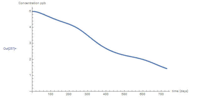
Proceeding iteratively produces the following graph with results almost identical to those produced by the explicit method. You can download the Microsoft Excel file example2implicit.xlsx showing the calculations.
 View Mathematica Code
ImplicitEulerMethod[fp_, x0_, h_, t0_, tmax_] :=
 (n = (tmax - t0)/h + 1;
  xtable = Table[0, {i, 1, n}];
  xtable[[1]] = x0;
  Do[s = FindRoot[x == xtable[[i - 1]] + h*fp[x, t0 + (i - 1) h], {x, xtable[[i - 1]]}]; xtable[[i]] = x /. s[[1]], {i, 2, n}];
  Data = Table[{t0 + (i - 1)*h, xtable[[i]]}, {i, 1, n}];
  Data)

f[t_] := 100 + 50*Cos[2 Pi*t/365];
cin[t_] := 5 E^(-2 t/1000);
fp[c_, t_] := f[t] (cin[t] - c)/10000;
Data = ImplicitEulerMethod[fp, 5, 1, 0, 365*2];
ListPlot[Data, AxesLabel -> {"time (days)", "Concentration ppb"}]
import numpy as np
import sympy as sp
import matplotlib.pyplot as plt

def ImplicitEulerMethod(fp, x0, h, t0, tmax):
  n = int((tmax - t0)/h + 1)
  xtable = [0 for i in range(n)]
  xtable[0] = x0
  x = sp.symbols('x')
  for i in range(1,n):
    s = sp.nsolve(x - xtable[i - 1] - h*fp(x, t0 + i*h), x, xtable[i - 1])
    xtable[i] = s
  Data = [[t0 + i*h, xtable[i]] for i in range(n)]
  return Data

def f(t): return 100 + 50*np.cos(2*np.pi*t/365)
def cin(t): return 5*np.exp(-2*t/1000)
def fp(c, t): return f(t)*(cin(t) - c)/10000
Data = ImplicitEulerMethod(fp, 5, 1, 0, 365*2)
plt.scatter([point[0] for point in Data],[point[1] for point in Data])
plt.xlabel("Time (days)"); plt.ylabel("Concentration ppb")
plt.grid(); plt.show()
Example 3
We will repeat Example 3 above to illustrate that the implicit Euler method is always stable.
Consider the IVP of the form:
![\[\frac{\mathrm{d}x}{\mathrm{d}t}=-x\]](https://engcourses-uofa.ca/wp-content/ql-cache/quicklatex.com-e562ee53adcc0c0b9f83a3ef66fcea90_l3.png "Rendered by QuickLaTeX.com")
If
 , compare the two solutions taking a step size of
  , and a step size of
  .
.
Solution
Using an implicit Euler scheme, the value of can be obtained as follows:
![\[x_{i+1}=x_i+h\frac{\mathrm{d}x}{\mathrm{d}t}\bigg|_{x_{i+1}}=x_i-h x_{i+1}\Rightarrow x_{i+1}=\frac{x_i}{(1+h)}=\frac{x_{i-1}}{(1+h)(1+h)}\]](https://engcourses-uofa.ca/wp-content/ql-cache/quicklatex.com-d467476e1392d14234a9edfe6d35a4cc_l3.png "Rendered by QuickLaTeX.com")
Therefore:
![\[x_{i+1}=\frac{x_0}{(1+h)^{i+1}}\]](https://engcourses-uofa.ca/wp-content/ql-cache/quicklatex.com-d3581d1140e25867e66b81979e75c0c3_l3.png "Rendered by QuickLaTeX.com")
is a positive number. Therefore, the term  is bounded for every
  and therefore, is bounded. The following tool illustrates the difference between the obtained result for
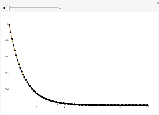
 ![t\in[0,10]](https://engcourses-uofa.ca/wp-content/ql-cache/quicklatex.com-ff10d62e92b48bda015872665c24c655_l3.png "Rendered by QuickLaTeX.com") . Vary the value of and notice how the obtained solution (black dots) compares to the exact solution (blue curve). While the accuracy is lost with higher values of , the solution maintains numerical stability.
. Vary the value of and notice how the obtained solution (black dots) compares to the exact solution (blue curve). While the accuracy is lost with higher values of , the solution maintains numerical stability.
Example 4
Consider the following nonlinear IVP:
![\[\frac{\mathrm{d}x}{\mathrm{d}t}=tx^2+2x\]](https://engcourses-uofa.ca/wp-content/ql-cache/quicklatex.com-bcd6500b414f07646b851aceb7ff00ed_l3.png "Rendered by QuickLaTeX.com")
with the initial condition  . Find the values of for
 ![t\in[0,5]](https://engcourses-uofa.ca/wp-content/ql-cache/quicklatex.com-89b22c375e995ed042c407a9d648430b_l3.png "Rendered by QuickLaTeX.com") taking using the implicit Euler method.
taking using the implicit Euler method.
Solution
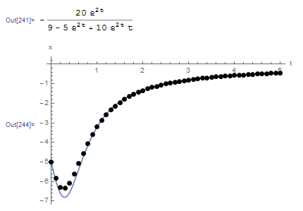
Using Mathematica, the exact solution to the differential equation given can be obtained as:
![\[x=\frac{-20e^{2t}}{9-5e^{2t}+10e^{2t}t}\]](https://engcourses-uofa.ca/wp-content/ql-cache/quicklatex.com-d2ad2bb80b845e0642f6b084483ed6a2_l3.png "Rendered by QuickLaTeX.com")
The implicit Euler scheme provides the following estimate for :
![\[x_{i+1}=x_i+h\frac{\mathrm{d}x}{\mathrm{d}t}\bigg|_{x=x_{i+1},t=t_{i+1}}=x_i+h(t_{i+1}x_{i+1}^2+2x_{i+1})\]](https://engcourses-uofa.ca/wp-content/ql-cache/quicklatex.com-48402b959e1ac90d4e9229f228b482f3_l3.png "Rendered by QuickLaTeX.com")
Since appears on both sides, and the equation is nonlinear in , therefore, the Newton-Raphson method will be used at each time increment to find the value of !
Setting  , , , and
  yields:
![\[x_1=-5+0.1(0.1 x_1^2+2x_1)\]](https://engcourses-uofa.ca/wp-content/ql-cache/quicklatex.com-2353b1a03386e4b34bfb9fdef0446af2_l3.png "Rendered by QuickLaTeX.com")
Solving the above nonlinear equation in  using the Newton-Raphson method yields:
![\[x_1=-5.82576\]](https://engcourses-uofa.ca/wp-content/ql-cache/quicklatex.com-e6b59018aafe7da6e552b10cf4b29ea2_l3.png "Rendered by QuickLaTeX.com")
Similarly, with  , the equation for is:
![\[x_2=-5.82576+0.1(0.2x_2^2+2x_2)\]](https://engcourses-uofa.ca/wp-content/ql-cache/quicklatex.com-a466aee3c571ad35a5e24e23b0ccf0be_l3.png "Rendered by QuickLaTeX.com")
Using the Newton-Raphson method:
![\[x_2=-6.29235\]](https://engcourses-uofa.ca/wp-content/ql-cache/quicklatex.com-244b303196937a0f733d33e06a359e2b_l3.png "Rendered by QuickLaTeX.com")
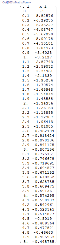
Proceeding iteratively produces the following table:
The following is the plot of the exact solution (blue line) with the data obtained using the implicit Euler method. The Mathematica code is given below.
 View Mathematica Code
ImplicitEulerMethod[fp_, x0_, h_, t0_, tmax_] :=
(n = (tmax - t0)/h + 1;
  xtable = Table[0, {i, 1, n}];
  xtable[[1]] = x0;
  Do[s = FindRoot[x == xtable[[i - 1]] + h*fp[x, t0 + (i - 1) h], {x, xtable[[i - 1]]}]; xtable[[i]] = x /. s[[1]], {i, 2, n}];
  Data2 = Table[{t0 + (i - 1)*h, xtable[[i]]}, {i, 1, n}];
  Data2)

Clear[x, xtable]
a = DSolve[{x'[t] == t*x[t]^2 + 2*x[t], x[0] == -5}, x, t];
x = x[t] /. a[[1]]
fp[x_, t_] := t*x^2 + 2*x;
Data2 = ImplicitEulerMethod[fp, -5.0, 0.1, 0, 5];
Plot[x, {t, 0, 5}, Epilog -> {PointSize[Large], Point[Data2]},AxesOrigin -> {0, 0}, AxesLabel -> {"t", "x"}, PlotRange -> All]
Title = {"t_i", "x_i"};
Data2 = Prepend[Data2, Title];
Data2 // MatrixForm
import numpy as np
import sympy as sp
import matplotlib.pyplot as plt
sp.init_printing(use_latex=True)

def ImplicitEulerMethod(fp, x0, h, t0, tmax):
  n = int((tmax - t0)/h + 1)
  xtable = [0 for i in range(n)]
  xtable[0] = x0
  x = sp.symbols('x')
  for i in range(1,n):
    s = sp.nsolve(x - xtable[i - 1] - h*fp(x, t0 + i*h), x, xtable[i - 1])
    xtable[i] = s
  Data = [[t0 + i*h, xtable[i]] for i in range(n)]
  return Data

x = sp.Function('x')
t = sp.symbols('t')
sol = sp.dsolve(x(t).diff(t) - t*x(t)**2 - 2*x(t), ics={x(0): -5})
display(sol)
def fp(x, t): return t*x**2 + 2*x
Data = ImplicitEulerMethod(fp, -5.0, 0.1, 0, 5)
x_val = np.arange(0,5,0.01)
plt.plot(x_val, [sol.subs(t, i).rhs for i in x_val])
plt.scatter([point[0] for point in Data],[point[1] for point in Data],c='k')
plt.xlabel("t"); plt.ylabel("x")
plt.grid(); plt.show()
print(["t_i", "x_i"],"\n",np.vstack(Data))
This was so helpful to me, thanks