Numerical Differentiation: Introduction

Introduction

Let be a smooth (differentiable) function, then the derivative of at is defined as the limit:

When is an explicit function of , one can often find an expression for the derivative of . For example, assuming is a polynomial function such that , then the derivative of is given by:

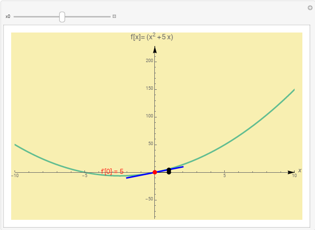
From a geometric perspective, the derivative of the function at a point gives the slope of the tangent to the function at that point. The following tool shows the slope () of the tangent to the function . You can move the slider to see how the slope changes. You can also download the code below and edit it to calculate the derivatives of any function you wish. This tool was created based on the Wolfram Demonstration Project of the derivative.

Clear[x, f, x0]
f[x_] := x^2 + 5 x;
xstart = -10;
xstop = 10;
Deltax = xstart - xstop;
Manipulate[
 kchangesides = xstart/2 + xstop/2;
 koffsetleft = 0.2 Deltax;
 koffsetright = 0.15 Deltax;
 ystop = Maximize[{f[x], xstart <= x <= xstop}, x][[1]];
 ystart = Minimize[{f[x], xstart <= x <= xstop}, x][[1]];
 Deltay = (ystop - ystart)*0.5;
 ystop = ystop + Deltay;
 ystart = ystart - Deltay;
 dx = (xstop - xstart)/10;
 funccolor = RGBColor[0.378912, 0.742199, 0.570321];
 Plot[{f[x]}, {x, xstart, xstop}, 
  PlotRange -> {{xstart, xstop}, {ystart, ystop}}, ImageSize -> 600, 
  AxesLabel -> {Style["x", 14, Italic], Style["f[x]=" f[x], 15]}, 
  Background -> RGBColor[0.972549, 0.937255, 0.694118], 
  PlotStyle -> {{funccolor, Thickness[.005]}}, 
  Epilog -> {Black, PointSize[.015], Arrowheads[.025], Arrow[{{xstop - .02, 0}, {xstop, 0}}], Arrow[{{0, ystop - .02}, {0, ystop}}], Line[{{x0, f[x0]}, {x0 + 1, f[x0]}}], Thickness[.005], Blue, Line[{{x0 - dx, f[x0] - dx f'[x0]}, {x0 + dx,  f[x0] + dx f'[x0]}}], Red, Point[{x0, f[x0]}], Line[{{x0 + 1, f[x0]}, {x0 + 1, f'[x0] + f[x0]}}], Black,  Point[{x0 + 1, f'[x0] + f[x0]}], Point[{x0 + 1, f[x0]}], Red,  Style[Inset[Row[{"f'[", x0, "] = ", ToString[NumberForm[N@f'[x0], {4, 3}]]}], If[x0 < kchangesides, {x0 - koffsetleft, f[x0]}, {x0 + koffsetright, f[x0]}]], 14]}], 
{x0, xstart, xstop}]

import numpy as np
import matplotlib.pyplot as plt
from ipywidgets.widgets import interact

def f(x): return x**2 + 5*x
def f_prime(x0, x): return (2*x0 + 5)*(x - x0) + f(x0)
@interact(x0=(-10,10,0.01))
def update(x0=-10):
  x = np.arange(-15, 15, 0.5)
  slope = (f_prime(x0, x0 + 1.5) - f(x0))/(1.5)
  plt.plot(x, f(x))
  plt.plot([x0 - 2, x0 + 2], [f_prime(x0, x0 - 2), f_prime(x0, x0 + 2)], linewidth=3)
  plt.plot([x0, x0 + 1.5],[f(x0), f(x0)])
  plt.plot([x0 + 1.5, x0 + 1.5],[f(x0), f_prime(x0, x0 + 1.5)])
  plt.text(x0, f(x0)+25, "f'("+str(x0)+") = "+str(round(slope,3)))
  plt.title("x**2 + 5x")
  plt.scatter([x0],[f(x0)],c='r')
  plt.xlim(-11,11); plt.ylim(-20, 170)
  plt.grid(); plt.show() 

The derivative of a function has many practical applications. Perhaps the most ubiquitous example is that of trying to calculate the velocity and the acceleration of a moving body if its position with respect to time is known. For example, one of our research projects in sports Biomechanics has focused on comparing the velocity and acceleration of squash players during tournament matches. To do so, the position of the player’s feet can be tracked on the court and then, using numerical differentiation, the velocity and acceleration can be quantified. The following video shows the tracked feet of a few rallies of one of the analyzed games:

In this case, and in many similar cases, there is no explicit function to be differentiated, and therefore, one has to deal with numerically differentiating the existing data. In other cases, an explicit formula for calculating the derivative might not exist and thus, if the derivative is sought, a numerical tool would be necessary.

Another similar interesting application is the estimation of the possible 100m time of Usain Bolt during the 2008 Beijing Olympics had he not celebrated in the last 20m during his race. Using some techniques described here along with some statistical analyses the authors of the article cited provide a good estimate of the time that Usain could have achieved.

Lecture Video