Engineering at Alberta Courses » Getting Started with Mathematica

Mathematica Lab Tutorials: Getting Started with Mathematica

This section covers the syntax and functions in Mathematica that are needed to solve the majority of the labs

Variables

Mathematica is symbolic and case sensitive. In the Mathematica notebook, you can write a few lines of code and then hit “Shift”+”Enter” to evaluate those lines. A semi-colon can be used to suppress the output from a particular line. Let’s try using an example. The following expression relates the variables $y$ and $x$ as follows:

$y=\frac{x^2(1+\sqrt{x})}{x+4}$

Mathematica is able to store that expression without evaluating either $y$ or $x$ :

y=x^2(1+Sqrt[x])/(x+4)

To evaluate $y$ when $x=2$ and when $x=3$ , there are two options. The first is to set $x=2$ and then type $y$ , then set $x=3$ and type $y$ as follows:

y=x^2(1+Sqrt[x])/(x+4)
x=2;
y
x=3;
y
x

Notice that when $x$ was assigned 2 and 3, the output was suppressed using a semi-colon. In this first option, the value of $x$ is set throughout the lines of the code and so if $x$ appears anywhere else it will adopt the most recent assigned value. Another option is to use evaluation rules. The following code evaluates $y$ when $x=2$ and then evaluates it again when $x=3$ . The variable $x$ itself is not assigned any value and so, when it appears afterwards, it is still unassigned:

y=x^2(1+Sqrt[x])/(x+4)
y/.x->2
y/.x->3
x
y

You can always use the “Clear” command to clear the variables before any operation. Also, note that in the second option, the evaluation of $y$ at $x=2$ was not stored in any variable but was just shown in the output. In the following code, the “Clear” command is used first to clear the variables, and then the evaluation of $y$ at $x=2$ is stored in the variable $z$ :

Clear[y,x]
y=x^2(1+Sqrt[x])/(x+4)
z=y/.x->2

Notice that after evaluating the previous lines of code, the variable $x$ appears in blue and the variable $y$ appears in black. Blue variables indicate that they are neither recognized functions in Mathematica, nor do they have any assigned values. The variable $y$ appears in black as it has been assigned the expression in the first line.

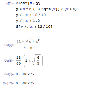
If only fractions and no decimal points are used, Mathematica uses arbitrary precision so, the square roots are not evaluated numerically. However, if decimal points are used Mathematica uses machine precision (around sixteen significant digits) and evaluates the expressions accordingly. The function $N[]$ in Mathematica can also be used to evaluate an expression using machine precision. See the following snapshot where $y$ is evaluated three times when $x=1.2$ . In the first time, $y$ is evaluated when $x=\frac{12}{10}$ and the square roots are not evaluated. The second time, $y$ is evaluated when $x=1.2$ and so Mathematica automatically reverts to machine precision. The third time, the function $N[]$ is used to evaluate the expression using machine precision:

Lab1

Matrices

The curly brackets {} are used in Mathematica to define vectors and matrices. For example, to define

$x=\left(\begin{array}{c}1\\2\\3\end{array}\right)$

you can simply write:

x={1,2,3}

You can view the output in “MatrixForm” as follows:

x={1,2,3};
x//MatrixForm

Note that you should not define a matrix and use the “MatrixForm” keyword in the same line. Otherwise, the variable $x$ will not contain a proper vector but rather will contain the “MatrixForm” generated image.

There are two ways by which a matrix can be defined. The first is by directly defining the components using curly brackets. For example, to define:

$M=\left(\begin{matrix}1 & 2 & 3\\ 4 & 5 & 6 \\ 7 & 8 & 9\end{matrix}\right)$

Each row in the matrix would be defined between two curly brackets, individual rows would be separated by commas, and finally a set of curly brackets is used to enclose the rows as follows:

M={{1,2,3},{4,5,6},{7,8,9}}
M//MatrixForm

The second way to define a matrix is using the “Table” command. The following command defines a table with 3 rows ( $i=1$ to $3$ ) and 4 columns ( $j=1$ to $4$ ). Each entry is equal to the number of the row multiplied by the number of the column:

S=Table[i*j,{i,1,3},{j,1,4}]
S//MatrixForm

The “.” character is used for the dot product and to multiply matrices by vectors:

M={{1,2,3},{4,5,6},{7,8,9}}
x={1,2,3}
y={4,5,6}
Print["The dot product between x and y is"]
x.y
Print["The multiplication of M and x yields z="]
z=M.x;
z//MatrixForm

The determinant, inverse, and transpose of the matrix

$M=\left(\begin{matrix}1 & 2\\ 3 & 4\end{matrix}\right)$

can be obtained as follows:

M={{1,2},{3,4}};
Print["Determinant of M:"]
t=Det[M]
Print["Inverse of M:"]
Nn=Inverse[M];
Nn//MatrixForm
Print["Transpose of M:"]
Mt=Transpose[M];
Mt//MatrixForm

Note in the above code that the symbol $N$ is reserved in Mathematica for the function that evaluates numerical expressions. Therefore, the variable $Nn$ was used for the inverse of $M$ .
In order to extract a particular entry from a matrix, a set of double square brackets will be used. For example, the following code defines a matrix $M$ and a vector $x$ and then displays the second row of $M$ , the entry in the second row and third column of $M$ , and the third entry in $x$ :

M={{11,12,13},{21,22,23},{31,32,33}};
x={1,2,3};
Print["The second row of M:"]
M[[2]]
Print["The entry in the second row and third column of M:"]
M[[2,3]]
Print["The third entry in x:"]
x[[3]]

You can perform a whole operation on one of the rows of a matrix. For example, we can take the second row of the matrix $M$ defined above, multiply it by 5, add the first row and store the result in the second row of $M$ . This can be done in one step as follows:

M={{11,12,13},{21,22,23},{31,32,33}};
M[[2]]=5*M[[2]]+M[[1]]
M//MatrixForm

You can also insert a row in a matrix. For example, the following code inserts the vector $b={1,2,3}$ as the third row in the matrix $M$ defined above and store the result in the matrix $M$ :

M={{11,12,13},{21,22,23},{31,32,33}};
b={1,2,3}
M=Insert[M,b,3]
M//MatrixForm

If on the other hand you want to store the $b={1,2,3}$ as the third column in $M$ , you can simply transpose $M$ first, use the insert command, and then transpose the output:

M={{11,12,13},{21,22,23},{31,32,33}};
b={1,2,3}
M=Transpose[Insert[Transpose[M],b,3]]
M//MatrixForm

You can also drop a row or a column in $M$ . To drop the third row, simply use the “Drop” command as follows:

M={{11,12,13},{21,22,23},{31,32,33}};
M=Drop[M,{3}]
M//MatrixForm

To drop the third column, simply transpose $M$ , drop the third row, and then transpose the result back:

M={{11,12,13},{21,22,23},{31,32,33}};
M=Transpose[Drop[Transpose[M],{3}]]
M//MatrixForm

Built-In Functions

There are numerous built-in functions in Mathematica. The arguments of these functions are entered using one set of square brackets. The first character in the function is usually a capital letter. Always remember that Mathematica is case sensitive, so, it can recognize Sin[20] but cannot recognize sin[20]. The following show the usage of the functions “Sin( $\pi$ )”, “Cos( $\frac{\pi}{3}$ )”, “Log(3)” which is the natural logarithm, “Factorial(10)=10!”, and “Cross[ $x$ , $y$ ]” which gives the cross product between the vectors ( $x$ , and $y$ ).

Sin[Pi]
Cos[Pi/3]
Log[3.]
10!
x = {1, 2, 3};
y = {1, 4, 5};
Cross[x, y]

The built-in function “Sum” can be used to evaluate the sum of a sequence of numbers. For example, consider the sequence with the terms:

$a_n=n^2-n$

Therefore:

$a_1=1-1=0 \qquad a_2=2^2-2=3 \qquad \cdots$

To find the sum of the first 10 terms using Mathematica is straightforward:

Sum[n^2-n,{n,1,10}]

If the infinite sum of the sequence exists, then Mathematica can evaluate it. For example, consider the sequence:

$a_n=\frac{1}{2^n}$

Then:

$a_1=1 \qquad a_2=\frac{1}{2} \qquad a_3=\frac{1}{8} \qquad \cdots$

The infinite sum can be found using Mathematica as follows:

Sum[1/2^n,{n,1,Infinity}]

As Mathematica is a “Mathematics” software, it can be used to calculate derivatives and integrals. For example, consider the relationship

$y=x^2$

The first derivative of $y$ is:

$\frac{\mathrm{d}y}{\mathrm{d}x}=2x$

The second derivative of $y$ is:

$\frac{\mathrm{d}^2y}{\mathrm{d}x^2}=2$

On the other hand, the integral of $y$ is:

$\int \!y \,\mathrm{d}x=\frac{x^3}{3} + C$

While the bounded integral of $y$ for $x=1$ to $x=2$ is:

$\int_{x=1}^{x=2} \! y \,\mathrm{d}x=\frac{x^3}{3}\bigg{|}_{x=2} - \frac{x^3}{3}\bigg{|}_{x=1}=\frac{7}{3}$

All this can be done in Mathematica (in that respective order) as follows:

y = x^2
D[y, x]
D[y, {x, 2}]
Integrate[y, x]
Integrate[y, {x, 1, 2}]

Note, however, that Mathematica does not add the constant of integration for the indefinite integral.

Two important functions that will be used throughout are “FullSimplify” and “Chop”. “FullSimplify” can be used to simplify expressions, for example

y = Sin[x] + 25 Sin[x] + (1 - 5 x)^2 + (3 - 8 x)^2
FullSimplify[y]

The “Chop” command can be used in numerical calculations to set numbers that are very small to be equal to zero.

Plotting

There are numerous ways to display plots in Mathematica. Here we will focus on two commands “Plot” and “ListPlot”. The first is a direct method to plot a relationship. Consider:

$y=\sin{x}+x$

We can plot this relationship on the domain $x\in[0,10]$ as follows:

y=Sin[x]+x;
Plot[y,{x,0,10}]

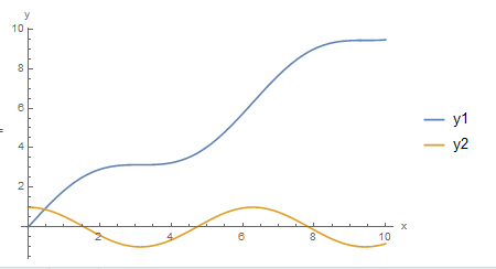
We can plot two different functions on the same plot, and we can use many options like adding a title, labels to the axes, and legend:

y1 = Sin[x] + x;
y2 = Cos[x];
Plot[{y1, y2}, {x, 0, 10}, AxesLabel -> {"x", "y"},AxesOrigin -> {0, 0}, PlotLegends -> {"y1", "y2"}]

The following is the produced plot
math2

The function “Show[]” can also combine multiple plots or graphics objects. You can visit the Mathematica Plot webpage to view the possible options that can be used to make your plots look professional. In particular, you always have to define the axes labels and the units (if known) for the variables used.

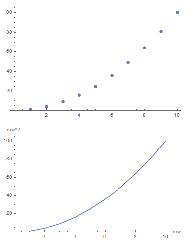
The second method for plotting is the “ListPlot”. This is used to plot data given in a table. For example, consider the $10\times 10$ table whose first column gives the row number (1 to 10) and the second column gives the row number squared:

a = Table[{i, i^2}, {i, 1, 10}];
a // MatrixForm

You can view the data using “ListPlot” as follows:

a = Table[{i, i^2}, {i, 1, 10}];
a // MatrixForm
ListPlot[a]
ListPlot[a, Joined -> True, AxesLabel -> {"row", "row^2"}]

The following are the two plots produced using the above commands. You can visit the Mathematica ListPlot webpage to view the possible options that can be used to make your plots look professional.
math3

Loops

There are different ways of constructing loops in Mathematica. We will be using “Do”, “While”, and “For”. The “Do” command evaluates an expression looping over a variable. For example, let’s define a vector $x$ of length 100 with zero entries:

x = Table[0, {i, 1, 100}];

We can then assign other values to the entries of the array $x$ using the “Do” command. For example, the following assigns the value $i^3$ to the entry number $i$ :

x = Table[0, {i, 1, 100}];
Do[x[[i]]=i^3,{i,1,100}]
x//MatrixForm

This could have been done in a different way using the “While” command as follows:

x = Table[0, {i, 1, 100}];
L=Length[x]
i=1;
While[i<=L,x[[i]]=i^3;i++]
x//MatrixForm

In the above example, $L$ is the length of the vector $x$ . The variable $i$ is set to 1. The “While” stores $i^3$ in the $i^{th}$ entry of $x$ and then adds 1 to $i$ using the expression $i++$ . The command is repeated while $i\leq L$ .

The “For” command can be used for the same thing as follows:

x = Table[0, {i, 1, 100}];
L=Length[x]
For[i=1,i<=L,i++,x[[i]]=i^3]
x//MatrixForm

In the above code, the “For” function starts with $i=1$ and keeps looping as long as $i\leq L$ while adding increments of 1 using the command $i++$ . For each value of $i$ , the $i^{th}$ entry of $x$ is set to $i^3$ .

The “For” command is very versatile, in the following code we start with $i=100$ , and keep looping as long as $i\geq 1$ . In each increment, we set $i=i-1$ . For each of $i$ , the $i^{th}$ entry of $x$ is set to $i^2$ .

x = Table[0, {i, 1, 100}];
L=Length[x]
For[i=100,i>=1,i=i-1,x[[i]]=i^2]
x//MatrixForm

User Defined Functions

User defined functions are useful tools to create specific functions that can be used throughout the code. Functions are defined using the symbols “:=”. The arguments of the function appear on the left hand side of the definition between a set of square brackets. Each argument is followed by the character “_”. The right hand side defines the calculations of the function and the output. For example, consider a function that squares its arguments. This would be defined as follows:

f[x_]:=x^2

Notice that the character “_” after “x” in the left hand side is used to indicate that “x” is local to the function. I.e., the variable “x” outside the function can take any other values. The following code defines the function “f” that squares its argument, then calls the function with argument 3, then calls the function with argument “y”, and then finally by typing “x” the output implies that the variable “x” is still undefined:

f[x_]:=x^2
f[3]
f[y]
x

A function can have multiple arguments or can have vectors or matrices as arguments. For example, the following code defines the trace function which returns the sum of the diagonal components of a matrix. Two matrices are then defined and then the function is called with these matrices as arguments.

g[M_] := Sum[M[[i, i]], {i, 1, Length[M]}]
A = {{1, 1}, {2, 1}};
B = {{1, 2, 3}, {4, 5, 6}, {7, 8, 9}};
g[A]
g[B]

The following function returns the sum of the first “i” terms in the vector “x”:

h[x_,i_] := Sum[x[[n]], {n, 1, i}]
y={1,2,3,4,5,6,7,8,9,10}
h[y,3]

You can define procedures using the function definition by using parentheses. For example, the following function takes a vector, calculates the number of components $n$ of the vector and then returns the sum of the elements 2 through $n$ .

Clear[n, h]
h[x_] := (n=Length[x];Sum[x[[i]], {i, 2, n}])
y={1,2,3,4,5,6,7,8,9,10}
h[y]

The procedure above can be defined using the keyword: “Module” which ensures that the variables within the procedure are not defined outside the procedure. In the example before, $n$ takes the value of 10 when the function $h(y)$ is called. Alternatively, the following code keeps $n$ undefined after the function is called:

Clear[n, h]
h[x_] := Module[{n},n=Length[x];Sum[x[[i]], {i, 2, n}]]
y={1,2,3,4,5,6,7,8,9,10}
h[y]
n

Solving Equations

Mathematica has built-in functions that can solve a multitude of equations. We will present the functions “Solve” and “DSolve”. Solve can be used to solve equations or inequalities. For example, consider the function:

$y=a_0 +a_1 x + a_2 x^2$

To find the values of $a_0$ , $a_1$ , and $a_2$ that would satisfy $y|_{x=1}=5$ , $y|_{x=2}=10$ , and $y|_{x=3}=25$ we can solve three equations in three unknowns as follows:

y=a0+a1*x+a2*x^2
Sol=Solve[{(y/.x->1)==5,(y/.x->2)==10,(y/.x->3)==25},{a0,a1,a2}]

Notice that two equal signs are used to differentiate from solving the equation and actually assigning values. Type the above in Mathematica and notice that the solution is given as a set of rules for $a_0$ , $a_1$ , and $a_2$ . To utilize these rules in the expression for $y$ you can type the following:

y=a0+a1*x+a2*x^2
Sol=Solve[{(y/.x->1)==5,(y/.x->2)==10,(y/.x->3)==25},{a0,a1,a2}]
y=y/.Sol[[1]]

The final outcome is that $y$ has the following expression:

$y=10-10x+5x^2$

Solve can also be used to solve nonlinear equations:

Clear[t]
Solve[-t^2 - t + 1 == 0, t]

The “DSolve” built-in function can be used to solve differential and algebraic equations. For example, consider the differential equation:

$y'=xy$

with the boundary condition $y[1]=1$ . The solution is $y=e^{\frac{x^2}{2}-\frac{1}{2}}$ . This solution can be obtained using the “DSolve” function as follows:

Clear[y]
sol = DSolve[{y'[x] == y[x]*x, y[1] == 1}, y[x], x]
y = y[x] /. sol[[1]]

Notice that the differential equation and the boundary conditions utilize the double equal characters and are inside a set of curly brackets. The last line in the code extracts the solution which is in the form of a rule and utilizes it to define the relationship for the variable $y$ .

Lab Problems

Consider the relationship
$y=\sin{\frac{\pi x}{6}}$

Find $y'$ and $y''$ . Evaluate $y$ , $y'$ , and $y''$ at $x_0=1$ . Then, plot the relationships $y$ , $y'$ , and $y''$ for the domain $x\in[-5,5]$ . Label your plot and plot legend appropriately.
Consider the sequence whose terms are $a_n=\frac{1}{3^n}$ . Evaluate the sum of the first twenty terms. Then, evaluate the infinite sum
$\sum_{n=1}^\infty a_n$

Use the ListPlot command to plot the first ten terms of the ordered pairs $(i,\sum_{n=1}^ia_n)$ . Label the plot appropriately and use the option “Joined->True”.
Consider the matrix
$M=\left(\begin{matrix}1 & x\\ x & 1\end{matrix}\right)$

Plot the relationship between the determinant of $M$ and $x$ for $x\in[-5,5]$ . Label the plot appropriately. From the plot, can you identify the values of $x$ for which the determinant is equal to zero?
The von Mises stress $\sigma_{vM}$ (or sometimes called equivalent stress) gives a positive measure of the state of stress given by the symmetric stress matrix:
$\sigma=\left(\begin{matrix}\sigma_{11} & \sigma_{12} & \sigma_{13} \\ \sigma_{12} & \sigma_{22} & \sigma_{23} \\ \sigma_{13} & \sigma_{23} & \sigma_{33} \end{matrix}\right)$

$\sigma_{vM}$ is defined as:

$\sigma_{vM}=\sqrt{\frac{(\sigma_{11}-\sigma_{22})^2+(\sigma_{22}-\sigma_{33})^2+(\sigma_{11}-\sigma_{33})^2+6(\sigma_{12}^2+\sigma_{13}^2+\sigma_{23}^2)}{2}}$

Create a function in Mathematica whose argument is a $3\times 3$ matrix and whose output is the von Mises stress. Use this function to show that the equivalent stress is the same for the following stress matrices (units of MPa):

$\sigma_a=\left(\begin{matrix}2&2&0\\2&5&0\\0&0&-5\end{matrix}\right)\qquad \sigma_b=\left(\begin{matrix}1&0&0\\0&-5&0\\0&0&6\end{matrix}\right)$
The $\cos(x)$ function where $x$ is in radian can be represented as the infinite series:
$\cos(x)=1-\frac{x^2}{2!}+\frac{x^4}{4!}-\cdots=\sum_{n=0}^{\infty}\frac{(-1)^n}{(2n)!}x^{2n}$

Let $i+1$ be the number of terms used to approximate the function $\cos(x)$ . Create a function in Mathematica whose inputs are $x$ and $i$ and whose output is the approximation:

$Approxcos(x,i)=\sum_{n=0}^{i}\frac{(-1)^n}{(2n)!}x^{2n}$

Show using numerical examples that your function gives proper approximations by comparing its output with the built-in $\cos$ function in Mathematica.
The $\sin(x)$ function where $x$ is in radian can be represented as the infinite series:
$\sin(x)=x-\frac{x^3}{3!}+\frac{x^5}{5!}-\frac{x^7}{7!}+\cdots = \sum_{n=0}^\infty\frac{(-1)^n}{(2n+1)!}x^{2n+1}$

Let $i+1$ be the number of terms used to approximate the function $\sin(x)$ . Create a function in Mathematica whose inputs are $x$ and $i$ and whose output is the approximation:

$Approxsin(x,i)=\sum_{n=0}^i\frac{(-1)^n}{(2n+1)!}x^{2n+1}$

Show using numerical examples that your function gives proper approximations by comparing its output with the built-in $\sin$ function in Mathematica.
The discharge velocity through an orifice at the bottom of a water tank open to the atmosphere is given by the relationship:

$v=\sqrt{2gh}$

where $h$ is the height of the water left in the tank. If $A_{orifice}$ is the “effective” area of the orifice and $A_{tank}$ is the cross sectional area of the tank, then the following differential equation describes the rate of change of the height of the water left in the tank

$\frac{\mathrm{d}h}{\mathrm{d}t}=-\frac{A_{orifice}}{A_{tank}}v$

Assuming that at $t=0$ the height of the water in the tank is given by $h_0$ , use the “DSolve function” to solve the above differential equation using Mathematica to find the height $h$ as a function of $A_{orifice}$ , $A_{tank}$ , $h_0$ , $g$ , and $t$ . Then, use the “Solve” function to show that the time $t_e$ to empty the tank (i.e., the time at which $h=0$ ) is given by the expression:

$t_e=\sqrt{\frac{2h_0}{g}}\frac{A_{tank}}{A_{orifice}}$
Write two functions in Mathematica whose arguments are a matrix and a vector. The first function should output the matrix after replacing the last row with the given vector. The second function should output the matrix after replacing the last column with the given vector.
Write a function in Mathematica whose inputs are another function $f$ and two values $a$ and $b$ . If $a<b$ , the output of the function should be the vector $\{a,b,f[a],f[b]\}$ , otherwise, the function should return the message: “Please ensure that a is less than b”. Show that this function works properly for different cases.
Use the “For” built-in function to create a function whose input is a vector of numbers. The function should check for the first occurrence of a number whose absolute value is less than 0.0005. The function should output the row number and that particular value. For example, if the input is the vector $v=\{1,3,2,5,0.1,0.2,-0.0004,0.03,0.000005\}$ , then the output should be $\{7,-0.0004\}$ . If none of the absolute values of the components of the vector is less than 0.0005, the function should output: “N/A”. Repeat the problem using the “While” built-in function.