
Numerical Integration: Gauss Quadrature
Gauss Quadrature
The Gauss integration scheme is a very efficient method to perform numerical integration over intervals. In fact, if the function to be integrated is a polynomial of an appropriate degree, then the Gauss integration scheme produces exact results. The Gauss integration scheme has been implemented in almost every finite element analysis software due to its simplicity and computational efficiency. This section outlines the basic principles behind the Gauss integration scheme. For its application to the finite element analysis method, please visit this section.
Introduction
Gauss quadrature aims to find the “least” number of fixed points to approximate the integral of a function ![f:[-1,1]\rightarrow \mathbb{R}](https://engcourses-uofa.ca/wp-content/ql-cache/quicklatex.com-b44be0e881a5cad1d59dd1a3856eeac5_l3.png "Rendered by QuickLaTeX.com") such that:
such that:
![\[ I=\int_{-1}^{1} \! f\,\mathrm{d}x \approx \sum_{i=1}^n w_i f(x_i) \]](https://engcourses-uofa.ca/wp-content/ql-cache/quicklatex.com-9adaa33f02ecc5f5cfa25d8a6d023502_l3.png "Rendered by QuickLaTeX.com")
where ![\forall 1\leq i\leq n:x_i\in[-1,1]](https://engcourses-uofa.ca/wp-content/ql-cache/quicklatex.com-280015c5c698df10daa92e01e4d76f99_l3.png "Rendered by QuickLaTeX.com") and
and  . Also,
  is called an integration point and
  is called the associated weight. The number of integration points and the associated weights are chosen according to the complexity of the function
  to be integrated. Since a general polynomial of degree
  has
has  coefficients, it is possible to find a Gauss integration scheme with
  number of integration points and number of associated weights to exactly integrate that polynomial function on the interval
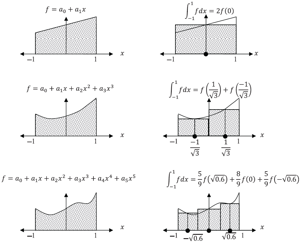
 ![[-1,1]](https://engcourses-uofa.ca/wp-content/ql-cache/quicklatex.com-4a7430a5619e08a23c430423c1376967_l3.png "Rendered by QuickLaTeX.com") . The following figure illustrates the concept of using the Gauss integration points to calculate the area under the curve for polynomials. In the following sections, the required number of integration points for particular polynomials are presented.
. The following figure illustrates the concept of using the Gauss integration points to calculate the area under the curve for polynomials. In the following sections, the required number of integration points for particular polynomials are presented.
Gauss Integration for Polynomials of the 1st, 3rd and 5th Degrees
Affine Functions (First-Degree Polynomials): One Integration Point
For a first-degree polynomial,  , therefore,
  , so, 1 integration point is sufficient as will be shown here. Consider
  with
with  , then:
![\[ \int_{-1}^{1} \! ax+b\,\mathrm{d}x=2b+a\frac{x^2}{2}\bigg|_{-1}^1=2b=2f(0) \]](https://engcourses-uofa.ca/wp-content/ql-cache/quicklatex.com-42598724c9bce16915b2fe2234930c73_l3.png "Rendered by QuickLaTeX.com")
So, for functions that are very close to being affine, a numerical integration scheme with 1 integration point that is  with an associated weight of 2 can be employed. In other words, a one-point numerical integration scheme has the form:
![\[ I=\int_{-1}^{1} \! f\,\mathrm{d}x \approx 2 f(0) \]](https://engcourses-uofa.ca/wp-content/ql-cache/quicklatex.com-140ab06e1479f22d19a13f9153c729ec_l3.png "Rendered by QuickLaTeX.com")
Third-Degree Polynomials: Two Integration Points
For a third-degree polynomial,  , therefore,
  , so, 2 integration points are sufficient as will be shown here. Consider
  , then:
![\[ \int_{-1}^{1} \! a_0+a_1x+a_2x^2+a_3x^3\,\mathrm{d}x=2a_0+2\frac{a_2}{3} \]](https://engcourses-uofa.ca/wp-content/ql-cache/quicklatex.com-588d17912294b3e4b0fce33b8eee7a44_l3.png "Rendered by QuickLaTeX.com")
Assuming 2 integration points in the Gauss integration scheme yields:
![\[ \int_{-1}^{1} \! a_0+a_1x+a_2x^2+a_3x^3\,\mathrm{d}x=w_1(a_0+a_1x_1+a_2x_1^2+a_3x_1^3)+w_2(a_0+a_1x_2+a_2x_2^2+a_3x_2^3) \]](https://engcourses-uofa.ca/wp-content/ql-cache/quicklatex.com-9fbfd96968875652a0d3f5b3146b9fd9_l3.png "Rendered by QuickLaTeX.com")
For the Gauss integration scheme to yield accurate results, the right-hand sides of the two equations above need to be equal for any choice of a cubic function. Therefore the multipliers of  ,
,  ,
,  , and
, and  should be the same. So, four equations in four unknowns can be written as follows:
![\[ \begin{split} w_1+w_2&=2\\ w_1x_1+w_2x_2&=0\\ w_1x_1^2+w_2x_2^2&=\frac{2}{3}\\ w_1x_1^3+w_2x_2^3&=0 \end{split} \]](https://engcourses-uofa.ca/wp-content/ql-cache/quicklatex.com-7acd5b30af7e2c531a452cc86be7a1af_l3.png "Rendered by QuickLaTeX.com")
The solution to the above four equations yields  ,
,  ,
,  . The Mathematica code below forms the above equations and solves them:
f = a0 + a1*x + a2*x^2 + a3*x^3;
I1 = Integrate[f, {x, -1, 1}]
I2 = w1*(f /. x -> x1) + w2*(f /. x -> x2)
Eq1 = Coefficient[I1 - I2, a0]
Eq2 = Coefficient[I1 - I2, a1]
Eq3 = Coefficient[I1 - I2, a2]
Eq4 = Coefficient[I1 - I2, a3]
Solve[{Eq1 == 0, Eq2 == 0, Eq3 == 0, Eq4 == 0}, {x1, x2, w1, w2}]
import sympy as sp
sp.init_printing(use_latex=True)
x, x1, x2 = sp.symbols('x x1 x2')
a0, a1, a2, a3 = sp.symbols('a0 a1 a2 a3')
w1, w2 = sp.symbols('w1 w2')
f = a0 + a1*x + a2*x**2 + a3*x**3
I1 = sp.integrate(f, (x, -1, 1))
I2 = w1*(f.subs(x, x1)) + w2*(f.subs(x, x2))
display("I1: ",I1)
display("I2: ",I2)
Eq1 = sp.expand(I1 - I2).coeff(a0)
Eq2 = sp.expand(I1 - I2).coeff(a1)
Eq3 = sp.expand(I1 - I2).coeff(a2)
Eq4 = sp.expand(I1 - I2).coeff(a3)
display("Eq1: ",Eq1)
display("Eq2: ",Eq2)
display("Eq3: ",Eq3)
display("Eq4: ",Eq4)
sol = list(sp.nonlinsolve([Eq1, Eq2, Eq3, Eq4], [x1, x2, w1, w2]))
display(sol)
So, for functions that are very close to being cubic, the following numerical integration scheme with 2 integration points can be employed:
![\[ I=\int_{-1}^{1} \! f\,\mathrm{d}x \approx f\left(\frac{-1}{\sqrt{3}}\right)+f\left(\frac{1}{\sqrt{3}}\right) \]](https://engcourses-uofa.ca/wp-content/ql-cache/quicklatex.com-4e2e3cd0f4f9a394e1dd4cc87ad07a36_l3.png "Rendered by QuickLaTeX.com")
Fifth-Degree Polynomials: Three Integration Points
For a fifth-degree polynomial,  , therefore,
  , so, 3 integration points are sufficient to exactly integrate a fifth-degree polynomial. Consider
  , then:
![\[ \int_{-1}^{1} \! a_0+a_1x+a_2x^2+a_3x^3+a_4x^4+a_5x^5\,\mathrm{d}x=2a_0+2\frac{a_2}{3}+2\frac{a_4}{5} \]](https://engcourses-uofa.ca/wp-content/ql-cache/quicklatex.com-d953ea0f7acca04c96dff423188e29a3_l3.png "Rendered by QuickLaTeX.com")
Assuming 3 integration points in the Gauss integration scheme yields:
![\[\begin{split} \int_{-1}^{1} \! &a_0+a_1x+a_2x^2+a_3x^3+a_4x^4+a_5x^5\,\mathrm{d}x=w_1(a_0+a_1x_1+a_2x_1^2+a_3x_1^3+a_4x_1^4+a_5x_1^5)\\ &+w_2(a_0+a_1x_2+a_2x_2^2+a_3x_2^3+a_4x_2^4+a_5x_2^5)+w_3(a_0+a_1x_3+a_2x_3^2+a_3x_3^3+a_4x_3^4+a_5x_3^5) \end{split} \]](https://engcourses-uofa.ca/wp-content/ql-cache/quicklatex.com-3c06a816f05dfc9ba4096e9dceb2ed82_l3.png "Rendered by QuickLaTeX.com")
For the Gauss integration scheme to yield accurate results, the right-hand sides of the two equations above need to be equal for any choice of a fifth-order polynomial function. Therefore the multipliers of , , , ,  , and
, and  should be the same. So, six equations in six unknowns can be written as follows:
![\[ \begin{split} w_1+w_2+w_3&=2\\ w_1x_1+w_2x_2+w_3x_3&=0\\ w_1x_1^2+w_2x_2^2+w_3x_3^2&=\frac{2}{3}\\ w_1x_1^3+w_2x_2^3+w_3x_3^3&=0\\ w_1x_1^4+w_2x_2^4+w_3x_3^4&=\frac{2}{5}\\ w_1x_1^5+w_2x_2^5+w_3x_3^5&=0 \end{split} \]](https://engcourses-uofa.ca/wp-content/ql-cache/quicklatex.com-079fb8f3210a619d9848a61fc7bd8051_l3.png "Rendered by QuickLaTeX.com")
The solution to the above six equations yields  ,
,  ,
,  ,
,  ,
,  , and
, and  . The Mathematica code below forms the above equations and solves them:
f = a0 + a1*x + a2*x^2 + a3*x^3 + a4*x^4 + a5*x^5;
I1 = Integrate[f, {x, -1, 1}]
I2 = w1*(f /. x -> x1) + w2*(f /. x -> x2) + w3*(f /. x -> x3)
Eq1 = Coefficient[I1 - I2, a0]
Eq2 = Coefficient[I1 - I2, a1]
Eq3 = Coefficient[I1 - I2, a2]
Eq4 = Coefficient[I1 - I2, a3]
Eq5 = Coefficient[I1 - I2, a4]
Eq6 = Coefficient[I1 - I2, a5]
Solve[{Eq1 == 0, Eq2 == 0, Eq3 == 0, Eq4 == 0, Eq5 == 0, Eq6 == 0}, {x1, x2, x3, w1, w2, w3}]
import sympy as sp
sp.init_printing(use_latex=True)
x, x1, x2, x3 = sp.symbols('x x1 x2 x3')
a0, a1, a2, a3, a4, a5 = sp.symbols('a0 a1 a2 a3 a4 a5')
w1, w2, w3 = sp.symbols('w1 w2 w3')
f = a0 + a1*x + a2*x**2 + a3*x**3 + a4*x**4 + a5*x**5
I1 = sp.integrate(f, (x, -1, 1))
I2 = w1*(f.subs(x, x1)) + w2*(f.subs(x, x2)) + w3*(f.subs(x, x3))
display("I1: ",I1)
display("I2: ",I2)
Eq1 = sp.expand(I1 - I2).coeff(a0)
Eq2 = sp.expand(I1 - I2).coeff(a1)
Eq3 = sp.expand(I1 - I2).coeff(a2)
Eq4 = sp.expand(I1 - I2).coeff(a3)
Eq5 = sp.expand(I1 - I2).coeff(a4)
Eq6 = sp.expand(I1 - I2).coeff(a5)
display("Eq1: ",Eq1)
display("Eq2: ",Eq2)
display("Eq3: ",Eq3)
display("Eq4: ",Eq4)
display("Eq5: ",Eq5)
display("Eq6: ",Eq6)
sol = list(sp.nonlinsolve([Eq1, Eq2, Eq3, Eq4, Eq5, Eq6], [x1, x2, x3, w1, w2, w3]))
display(sol)
So, for functions that are very close to being fifth-order polynomials, the following numerical integration scheme with 3 integration points can be employed:
![\[ I=\int_{-1}^{1} \! f\,\mathrm{d}x \approx \frac{5}{9}f\left(-\sqrt{\frac{3}{5}}\right)+\frac{8}{9}f(0)+\frac{5}{9}f\left(\sqrt{\frac{3}{5}}\right) \]](https://engcourses-uofa.ca/wp-content/ql-cache/quicklatex.com-967f03f737cbcb8b546f3755a1759bef_l3.png "Rendered by QuickLaTeX.com")
Seventh-Degree Polynomial: Four Integration Points
For a seventh-degree polynomial,  , therefore,
  , so, 4 integration points are sufficient to exactly integrate a seventh-degree polynomial. Following the procedure outlined above, the integration points along with the associated weight:
![\[\begin{split} x_1=-0.861136 \qquad w_1=0.347855\\ x_2=-0.339981 \qquad w_2=0.652145\\ x_3=0.339981 \qquad w_3=0.652145\\ x_4=0.861136 \qquad w_4=0.347855 \end{split} \]](https://engcourses-uofa.ca/wp-content/ql-cache/quicklatex.com-45e63564a6dd5756605d5fb69bb89c29_l3.png "Rendered by QuickLaTeX.com")
So, for functions that are very close to being seventh-order polynomials, the following numerical integration scheme with 4 integration points can be employed:
![\[\begin{split} I&=\int_{-1}^{1} \! f\,\mathrm{d}x\\ & \approx 0.347855f(-0.861136)+0.652145f(-0.339981)\\ & +0.652145f(0.339981)+0.347855f(0.861136) \end{split} \]](https://engcourses-uofa.ca/wp-content/ql-cache/quicklatex.com-7ef1e067e795fffd6bb0b612e96f6185_l3.png "Rendered by QuickLaTeX.com")
The following is the Mathematica code used to find the above integration points and corresponding weights.
View Mathematica Codef = a0 + a1*x + a2*x^2 + a3*x^3 + a4*x^4 + a5*x^5 + a6*x^6 + a7*x^7;
I1 = Integrate[f, {x, -1, 1}]
I2 = w1*(f /. x -> x1) + w2*(f /. x -> x2) + w3*(f /. x -> x3) + w4*(f /. x -> x4)
Eq1 = Coefficient[I1 - I2, a0]
Eq2 = Coefficient[I1 - I2, a1]
Eq3 = Coefficient[I1 - I2, a2]
Eq4 = Coefficient[I1 - I2, a3]
Eq5 = Coefficient[I1 - I2, a4]
Eq6 = Coefficient[I1 - I2, a5]
Eq7 = Coefficient[I1 - I2, a6]
Eq8 = Coefficient[I1 - I2, a7]
a = Solve[{Eq1 == 0, Eq2 == 0, Eq3 == 0, Eq4 == 0, Eq5 == 0, Eq6 == 0, Eq7 == 0, Eq8 == 0}, {x1, x2, x3, w1, w2, w3, x4, w4}]
Chop[N[a[[1]]]]
import sympy as sp
sp.init_printing(use_latex=True)
x, x1, x2, x3, x4 = sp.symbols('x x1 x2 x3 x4')
a0, a1, a2, a3, a4, a5, a6, a7 = sp.symbols('a0 a1 a2 a3 a4 a5 a6 a7')
w1, w2, w3, w4 = sp.symbols('w1 w2 w3 w4')
f = a0 + a1*x + a2*x**2 + a3*x**3 + a4*x**4 + a5*x**5 + a6*x**6 + a7*x**7
I1 = sp.integrate(f, (x, -1, 1)).subs({x3:-x1,x4:-x2,w3:w1,w4:w2})
I2 = (w1*(f.subs(x, x1)) + w2*(f.subs(x, x2)) + w3*(f.subs(x, x3)) +  w4*(f.subs(x, x4))).subs({x3:-x1,x4:-x2,w3:w1,w4:w2})
display("I1: ",I1)
display("I2: ",I2)
Eq1 = sp.expand(I1 - I2).coeff(a0)
Eq2 = sp.expand(I1 - I2).coeff(a1)
Eq3 = sp.expand(I1 - I2).coeff(a2)
Eq4 = sp.expand(I1 - I2).coeff(a3)
Eq5 = sp.expand(I1 - I2).coeff(a4)
Eq6 = sp.expand(I1 - I2).coeff(a5)
Eq7 = sp.expand(I1 - I2).coeff(a6)
Eq8 = sp.expand(I1 - I2).coeff(a7)
display("Eq1: ",Eq1)
display("Eq2: ",Eq2)
display("Eq3: ",Eq3)
display("Eq4: ",Eq4)
display("Eq5: ",Eq5)
display("Eq6: ",Eq6)
display("Eq7: ",Eq7)
display("Eq8: ",Eq8)
sol = list(sp.nonlinsolve([Eq1, Eq3, Eq5, Eq7], [x1, x2, w1, w2]))
display(sol)
Ninth-Degree Polynomial: Five Integration Points
For a ninth-degree polynomial,  , therefore,
  , so, 5 integration points are sufficient to exactly integrate a ninth-degree polynomial. Following the procedure outlined above, the integration points along with the associated weight:
![\[\begin{split} x_1=-0.90618 \qquad w_1=0.236927\\ x_2=-0.538469 \qquad w_2=0.478629\\ x_3=0 \qquad w_3=0.568889\\ x_4=0.538469 \qquad w_4=0.478629\\ x_5=0.90618 \qquad w_5=0.236927 \end{split} \]](https://engcourses-uofa.ca/wp-content/ql-cache/quicklatex.com-70074209cd7d5d45f3ad78d9e28a4f31_l3.png "Rendered by QuickLaTeX.com")
So, for functions that are very close to being ninth-order polynomials, the following numerical integration scheme with 5 integration points can be employed:
![\[\begin{split} I&=\int_{-1}^{1} \! f\,\mathrm{d}x\\ & \approx 0.236927f(-0.90618)+0.478629f(-0.538469)\\ & +0.568889f(0)+0.478629f(0.538469)\\ & + 0.236927 f(0.90618) \end{split} \]](https://engcourses-uofa.ca/wp-content/ql-cache/quicklatex.com-053256c5108eadf390d18e603028c575_l3.png "Rendered by QuickLaTeX.com")
The following is the Mathematica code used to find the above integration points and corresponding weights.
View Mathematica Codef = a0 + a1*x + a2*x^2 + a3*x^3 + a4*x^4 + a5*x^5 + a6*x^6 + a7*x^7 + a8*x^8 + a9*x^9;
I1 = Integrate[f, {x, -1, 1}]
I2 = w1*(f /. x -> x1) + w2*(f /. x -> x2) + w3*(f /. x -> x3) + w4*(f /. x -> x4) + w5*(f /. x -> x5)
Eq1 = Coefficient[I1 - I2, a0]
Eq2 = Coefficient[I1 - I2, a1]
Eq3 = Coefficient[I1 - I2, a2]
Eq4 = Coefficient[I1 - I2, a3]
Eq5 = Coefficient[I1 - I2, a4]
Eq6 = Coefficient[I1 - I2, a5]
Eq7 = Coefficient[I1 - I2, a6]
Eq8 = Coefficient[I1 - I2, a7]
Eq9 = Coefficient[I1 - I2, a8]
Eq10 = Coefficient[I1 - I2, a9]
a = Solve[{Eq1 == 0, Eq2 == 0, Eq3 == 0, Eq4 == 0, Eq5 == 0, Eq6 == 0, Eq7 == 0, Eq8 == 0, Eq9 == 0, Eq10 == 0}, {x1, x2, x3, w1, w2, w3, x4, w4, x5, w5}]
Chop[N[a[[1]]]]
import sympy as sp
sp.init_printing(use_latex=True)
x, x1, x2, x3, x4, x5 = sp.symbols('x x1 x2 x3 x4 x5')
a0, a1, a2, a3, a4, a5, a6, a7, a8, a9 = sp.symbols('a0 a1 a2 a3 a4 a5 a6 a7 a8 a9')
w1, w2, w3, w4, w5 = sp.symbols('w1 w2 w3 w4 w5')
f = a0 + a1*x + a2*x**2 + a3*x**3 + a4*x**4 + a5*x**5 + a6*x**6 + a7*x**7 + a8*x**8 + a9*x**9
I1 = sp.integrate(f, (x, -1, 1)).subs({x3:-x1,x4:-x2,x5:0,w3:w1,w4:w2})
I2 = (w1*(f.subs(x, x1)) + w2*(f.subs(x, x2)) + w3*(f.subs(x, x3)) +   w4*(f.subs(x, x4)) + w5*(f.subs(x, x5))).subs({x3:-x1,x4:-x2,x5:0,w3:w1,w4:w2})
display("I1: ",I1)
display("I2: ",I2)
Eq1 = sp.expand(I1 - I2).coeff(a0)
Eq2 = sp.expand(I1 - I2).coeff(a1)
Eq3 = sp.expand(I1 - I2).coeff(a2)
Eq4 = sp.expand(I1 - I2).coeff(a3)
Eq5 = sp.expand(I1 - I2).coeff(a4)
Eq6 = sp.expand(I1 - I2).coeff(a5)
Eq7 = sp.expand(I1 - I2).coeff(a6)
Eq8 = sp.expand(I1 - I2).coeff(a7)
Eq9 = sp.expand(I1 - I2).coeff(a8)
Eq10 = sp.expand(I1 - I2).coeff(a9)
display("Eq1: ",Eq1)
display("Eq2: ",Eq2)
display("Eq3: ",Eq3)
display("Eq4: ",Eq4)
display("Eq5: ",Eq5)
display("Eq6: ",Eq6)
display("Eq7: ",Eq7)
display("Eq8: ",Eq8)
display("Eq9: ",Eq9)
display("Eq10: ",Eq10)
sol = list(sp.nonlinsolve([Eq1, Eq3, Eq5, Eq7, Eq9], [x1, x2, w1, w2, w5]))
display(sol)
Eleventh-Degree Polynomial: Six Integration Points
For an eleventh-degree polynomial,  , therefore,
  , so, 6 integration points are sufficient to exactly integrate an eleventh-degree polynomial. Following the procedure outlined above, the integration points along with the associated weight:
![\[\begin{split} x_1=-0.93247 \qquad w_1=0.171324\\ x_2=-0.661209 \qquad w_2=0.360762\\ x_3=-0.238619 \qquad w_3=0.467914\\ x_4=0.238619 \qquad w_4=0.467914\\ x_5=0.661209 \qquad w_5=0.360762\\ x_6=0.93247 \qquad w_6=0.171324\\ \end{split} \]](https://engcourses-uofa.ca/wp-content/ql-cache/quicklatex.com-a0030a33255bb167e53520bcd05a6476_l3.png "Rendered by QuickLaTeX.com")
So, for functions that are very close to being eleventh-order polynomials, the following numerical integration scheme with 6 integration points can be employed:
![\[\begin{split} I&=\int_{-1}^{1} \! f\,\mathrm{d}x\\ & \approx 0.171324f(-0.93247 )+0.360762f(-0.661209 )\\ & +0.467914f(-0.238619)+0.467914f(0.238619)\\ & + 0.360762f(0.661209 )+0.171324f(0.93247 ) \end{split} \]](https://engcourses-uofa.ca/wp-content/ql-cache/quicklatex.com-d2bf620ef2d07461c9ea37101ea7f555_l3.png "Rendered by QuickLaTeX.com")
The following is the Mathematica code used to find the above integration points and corresponding weights. Note that symmetry was employed to reduce the number of equations.
View Mathematica Codef = a0 + a1*x + a2*x^2 + a3*x^3 + a4*x^4 + a5*x^5 + a6*x^6 + a7*x^7 + a8*x^8 + a9*x^9 + a10*x^10 + a11*x^11;
I1 = Integrate[f, {x, -1, 1}]
I2 = w1*(f /. x -> x1) + w2*(f /. x -> x2) + w3*(f /. x -> x3) +
w3*(f /. x -> -x3) + w2*(f /. x -> -x2) + w1*(f /. x -> -x1)
Eq1 = Coefficient[I1 - I2, a0]
Eq3 = Coefficient[I1 - I2, a2]
Eq5 = Coefficient[I1 - I2, a4]
Eq7 = Coefficient[I1 - I2, a6]
Eq9 = Coefficient[I1 - I2, a8]
Eq11 = Coefficient[I1 - I2, a10]
a = Solve[{Eq1 == 0, Eq3 == 0, Eq5 == 0, Eq7 == 0, Eq9 == 0, Eq11 == 0}, {x1, x2, x3, w1, w2, w3}]
Chop[N[a[[1]]]]
import numpy as np
import sympy as sp
from scipy.optimize import fsolve
sp.init_printing(use_latex=True)

x, x1, x2, x3 = sp.symbols('x x1 x2 x3')
a0, a1, a2, a3, a4, a5, a6, a7, a8, a9, a10, a11 = sp.symbols('a0 a1 a2 a3 a4 a5 a6 a7 a8 a9 a10 a11')
w1, w2, w3, w4, w5 = sp.symbols('w1 w2 w3 w4 w5')
f = a0 + a1*x + a2*x**2 + a3*x**3 + a4*x**4 + a5*x**5 + a6*x**6 + a7*x**7 + a8*x**8 + a9*x**9 + a10*x**10 + a11*x**11
I1 = sp.integrate(f, (x, -1, 1))
I2 =  w1*(f.subs(x, x1)) + w2*(f.subs(x, x2)) + w3*(f.subs(x, x3)) + w3*(f.subs(x, -x3)) + w2*(f.subs(x, -x2)) + w1*(f.subs(x, -x1))
display("I1: ",I1)
display("I2: ",I2)
Eq1 = sp.expand(I1 - I2).coeff(a0)
Eq2 = sp.expand(I1 - I2).coeff(a1)
Eq3 = sp.expand(I1 - I2).coeff(a2)
Eq4 = sp.expand(I1 - I2).coeff(a3)
Eq5 = sp.expand(I1 - I2).coeff(a4)
Eq6 = sp.expand(I1 - I2).coeff(a5)
Eq7 = sp.expand(I1 - I2).coeff(a6)
Eq8 = sp.expand(I1 - I2).coeff(a7)
Eq9 = sp.expand(I1 - I2).coeff(a8)
Eq10 = sp.expand(I1 - I2).coeff(a9)
Eq11 = sp.expand(I1 - I2).coeff(a10)
display("Eq1: ",Eq1)
display("Eq2: ",Eq2)
display("Eq3: ",Eq3)
display("Eq4: ",Eq4)
display("Eq5: ",Eq5)
display("Eq6: ",Eq6)
display("Eq7: ",Eq7)
display("Eq8: ",Eq8)
display("Eq9: ",Eq9)
display("Eq10: ",Eq10)
display("Eq11: ",Eq11)

# Convert Sympy equations to a Python function using lambdify
Equations = sp.lambdify(([x1, x2, x3, w1, w2, w3],), [Eq1, Eq3, Eq5, Eq7, Eq9, Eq11])
# Solve system of equations using Scipy's fsolve
sol = fsolve(Equations, [-0.5,-1,-0.3,0,0,0])
display(sol)
We can continue determining more integration points (abscissae) and weights for Gauss quadrature. In this page, the integration points and weights up to 64 points are available. Note that 64 integration points of Gauss quadrature is associated with a polynomial of degree 127.
Implementation of Gauss Quadrature
Gauss quadrature is very easy to implement and provides very accurate results with very few computations. However, one drawback is that it is not applicable to data obtained experimentally as the values of the function at the specific integration points would not be necessarily available. In order to implement the Gauss integration scheme in Mathematica, first, the following table is created which contains the integration points and the corresponding weights. Row number  contains the Gauss integration scheme with
  integration points. Then, a procedure is created in Mathematica whose input is a function , and the requested number of integration points. The procedure then calls the appropriate row in the “GaussTable” and calculates the weighted sum of the function evaluated at the appropriate integration points.
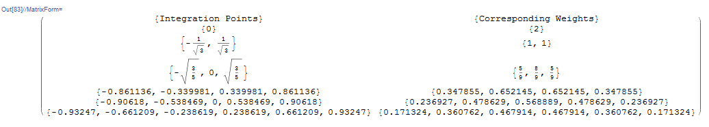
Clear[f, x]
GaussTable = {{{"Integration Points"}, {"Corresponding Weights"}}, {{0}, {2}}, {{-1/Sqrt[3], 1/Sqrt[3]}, {1, 1}}, {{-Sqrt[3/5], 0, Sqrt[3/5]}, {5/9, 8/9, 5/9}}, {{-0.861136, -0.339981, 0.339981, 0.861136}, {0.347855, 0.652145, 0.652145, 0.347855}}, {{-0.90618, -0.538469, 0, 0.538469, 0.90618}, {0.236927, 0.478629, 0.568889, 0.478629, 0.236927}}, {{-0.93247, -0.661209, -0.238619, 0.238619, 0.661209, 0.93247}, {0.171324, 0.360762, 0.467914, 0.467914, 0.360762,  0.171324}}};
GaussTable // MatrixForm
IG[f_, n_] := Sum[GaussTable[[n + 1, 2, i]]*f[GaussTable[[n + 1, 1, i]]], {i, 1, n}]
f[x_] := x^9 + x^8
IG[f, 5.0]
import numpy as np
import pandas as pd
GaussTable = [[[0], [2]], [[-1/np.sqrt(3), 1/np.sqrt(3)], [1, 1]], [[-np.sqrt(3/5), 0, np.sqrt(3/5)], [5/9, 8/9, 5/9]], [[-0.861136, -0.339981, 0.339981, 0.861136], [0.347855, 0.652145, 0.652145, 0.347855]], [[-0.90618, -0.538469, 0, 0.538469, 0.90618], [0.236927, 0.478629, 0.568889, 0.478629, 0.236927]], [[-0.93247, -0.661209, -0.238619, 0.238619, 0.661209, 0.93247], [0.171324, 0.360762, 0.467914, 0.467914, 0.360762,  0.171324]]]
display(pd.DataFrame(GaussTable, columns=["Integration Points", "Corresponding Weights"]))
def IG(f, n):
  n = int(n)
  return sum([GaussTable[n - 1][1][i]*f(GaussTable[n - 1][0][i]) for i in range(n)])
def f(x): return x**9 + x**8
IG(f, 5.0)
Example
Calculate the exact integral of  on the interval and find the relative error if a Gauss 1, 2, 3, and 4 integration points scheme is used. Also, calculate the number of rectangles required by the midpoint rule of the rectangle method to produce an error similar to that produced by the 3 point integration scheme, then evaluate the integral using the midpoint rule of the rectangle method with the obtained number of rectangles.
Solution
The exact integral is given by:
![\[ I=\int_{-1}^{1}\!\cos{x}\,\mathrm{d}x=\sin{(1)}-\sin{(-1)}=1.68294 \]](https://engcourses-uofa.ca/wp-content/ql-cache/quicklatex.com-411d1a03d3721da1944a209774229637_l3.png "Rendered by QuickLaTeX.com")
Employing a Gauss integration scheme with one integration point yields:
![\[\begin{split} I_1&=w_1\cos{x_1}=2 \cos{(0)}=2\\ E_r&=\frac{1.68294-2}{1.68294}=-0.1884 \end{split} \]](https://engcourses-uofa.ca/wp-content/ql-cache/quicklatex.com-f871bfb56b2deff0815944cefebe41b9_l3.png "Rendered by QuickLaTeX.com")
Employing a Gauss integration scheme with two integration points yields:
![\[ \begin{split} I_2&=w_1\cos{x_1}+w_2\cos{x_2}=\cos{\left(\frac{-1}{\sqrt{3}}\right)}+\cos{\left(\frac{1}{\sqrt{3}}\right)}=1.67582\\ E_r&=\frac{1.68294-1.67582}{1.68294}=0.00422968 \end{split} \]](https://engcourses-uofa.ca/wp-content/ql-cache/quicklatex.com-32caa2476d3464e03e8141b99e407065_l3.png "Rendered by QuickLaTeX.com")
Employing a Gauss integration scheme with three integration points yields:
![\[\begin{split} I_3&=w_1\cos{x_1}+w_2\cos{x_2}+w_3\cos{x_3}=\frac{5}{9}\cos{\left(-\sqrt{\frac{3}{5}}\right)}+\frac{8}{9}\cos{(0)}+\frac{5}{9}\cos{\left(\sqrt{\frac{3}{5}}\right)}=1.683\\ E_r&=\frac{1.68294-1.683}{1.68294}=-0.0003659 \end{split} \]](https://engcourses-uofa.ca/wp-content/ql-cache/quicklatex.com-b5c7c72a6720733f903c8511a9eaeb5c_l3.png "Rendered by QuickLaTeX.com")
Employing a Gauss integration scheme with four integration points yields:
![\[\begin{split} I_4&=w_1\cos{x_1}+w_2\cos{x_2}+w_3\cos{x_3}+w_4\cos{x_4}\\ &= 0.347855\cos(-0.861136)+0.652145\cos(-0.339981)\\ &+0.652145\cos(0.339981)+0.347855\cos(0.861136)\\ &=1.68294\\ E_r&=\frac{1.68294-1.68294}{1.68294}=0 \end{split} \]](https://engcourses-uofa.ca/wp-content/ql-cache/quicklatex.com-3ba045ee209d628ff6bab12db3ba324a_l3.png "Rendered by QuickLaTeX.com")
Using a three point integration scheme yielded an error of:
![\[ |E|=|1.68294-1.683| = |-0.00006|=0.00006 \]](https://engcourses-uofa.ca/wp-content/ql-cache/quicklatex.com-5db8c84e888ed0ed9ececfd183ddeda3_l3.png "Rendered by QuickLaTeX.com")
Equating the upper bound for the error in the midpoint rule to the error produced by a three-point Gauss integration scheme yields:
![\[ \max_{\xi\in[a,b]}|f''(\xi)| (b-a)\frac{h^2}{24}=0.00006 \]](https://engcourses-uofa.ca/wp-content/ql-cache/quicklatex.com-f6df0dbe7737379b80e42192bbaf2bf2_l3.png "Rendered by QuickLaTeX.com")
With  , and
, and ![\max_{\xi\in[a,b]}|f''(\xi)|=1](https://engcourses-uofa.ca/wp-content/ql-cache/quicklatex.com-19a68e3a4230df3f1dd7ed409251ea7a_l3.png "Rendered by QuickLaTeX.com") . Therefore:
. Therefore:
![\[ h=\sqrt{\frac{0.00006\times 24}{2}}=0.02683 \]](https://engcourses-uofa.ca/wp-content/ql-cache/quicklatex.com-5bc61f14f58f49f7447da4273559c8e8_l3.png "Rendered by QuickLaTeX.com")
Therefore, the required number of rectangles is:
![\[ n=\frac{b-a}{h}=\frac{2}{0.02683}\approx 75 \]](https://engcourses-uofa.ca/wp-content/ql-cache/quicklatex.com-a2c8417b5e8a49b2f6b840f81c4dfc4e_l3.png "Rendered by QuickLaTeX.com")
With 75 rectangles the rectangle method yields an integral of  . It is important to note how accurate the Gauss integration scheme is compared to the rectangle method. For this example, it would take 75 divisions (equivalent to 75 integration points) to reach an accuracy similar to the Gauss integration scheme with only 3 points!
Clear[f, x, I2]
GaussTable = {{{"Integration Points"}, {"Corresponding Weights"}}, {{0}, {2}}, {{-1/Sqrt[3], 1/Sqrt[3]}, {1, 1}}, {{-Sqrt[3/5], 0,  Sqrt[3/5]}, {5/9, 8/9, 5/9}}, {{-0.861136, -0.339981, 0.339981, 0.861136}, {0.347855, 0.652145, 0.652145, 0.347855}}, {{-0.90618, -0.538469, 0, 0.538469, 0.90618}, {0.236927, 0.478629, 0.568889, 0.478629, 0.236927}}, {{-0.93247, -0.661209, -0.238619, 0.238619, 0.661209, 0.93247}, {0.171324, 0.360762, 0.467914, 0.467914, 0.360762,  0.171324}}};
GaussTable // MatrixForm
IG[f_, n_] := Sum[GaussTable[[n + 1, 2, i]]*f[GaussTable[[n + 1, 1, i]]], {i, 1,  n}];
f[x_] := Cos[x]
Iexact = Integrate[Cos[x], {x, -1, 1.0}]
Itable = Table[{i, N[IG[f, i]], (Iexact - IG[f, i])/Iexact}, {i, 1, 6}];
Title = {"Number of Integration Points",  "Numerical Integration Results", "Relative Error"};
Itable = Prepend[Itable, Title];
Itable // MatrixForm
h = Sqrt[0.00006*24/2/1]
n = Ceiling[2/h]
I2[f_, a_, b_, n_] := (h = (b - a)/n; Sum[f[a + (i - 1/2)*h]*h, {i, 1, n}])
I2[f, -1.0, 1, n]
import numpy as np
import sympy as sp
import pandas as pd
from scipy import integrate

GaussTable = [[[0], [2]], [[-1/np.sqrt(3), 1/np.sqrt(3)], [1, 1]], [[-np.sqrt(3/5), 0, np.sqrt(3/5)], [5/9, 8/9, 5/9]], [[-0.861136, -0.339981, 0.339981, 0.861136], [0.347855, 0.652145, 0.652145, 0.347855]], [[-0.90618, -0.538469, 0, 0.538469, 0.90618], [0.236927, 0.478629, 0.568889, 0.478629, 0.236927]], [[-0.93247, -0.661209, -0.238619, 0.238619, 0.661209, 0.93247], [0.171324, 0.360762, 0.467914, 0.467914, 0.360762,  0.171324]]]
display(pd.DataFrame(GaussTable, columns=["Integration Points", "Corresponding Weights"]))
def IG(f, n):
  n = int(n)
  return sum([GaussTable[n - 1][1][i]*f(GaussTable[n - 1][0][i]) for i in range(n)])
def f(x): return np.cos(x)
Iexact, error = integrate.quad(f, -1, 1)
print("Iexact: ",Iexact)
Itable = [[i + 1, sp.N(IG(f, i + 1)), (Iexact - IG(f, i + 1))/Iexact] for i in range(6)]
Itable = pd.DataFrame(Itable, columns=["Number of Integration Points",  "Numerical Integration Results", "Relative Error"])
display(Itable)
h = np.sqrt(0.00006*24/2/1)
print("h: ",h)
n = np.ceil(2/h)
print("n: ",n)
def I2(f, a, b, n):
  h = (b - a)/n
  return sum([f(a + (i + 1/2)*h)*h for i in range(int(n))])
I2(f, -1.0, 1, n)
Alternate Integration Limits
The Gauss integration scheme presented above applies to functions that are integrated over the interval . A simple change of variables can be used to allow integrating a function  where
where ![z\in[a,b]](https://engcourses-uofa.ca/wp-content/ql-cache/quicklatex.com-0df50d7343f494f1f6b9ccd9ee9ad2e8_l3.png "Rendered by QuickLaTeX.com") . In this case, the linear relationship between
. In this case, the linear relationship between  and
and  can be expressed as:
![\[ \frac{z-a}{b-a}=\frac{x-(-1)}{1-(-1)}=\frac{x+1}{2} \]](https://engcourses-uofa.ca/wp-content/ql-cache/quicklatex.com-a4e8036b754090df2c3a9adf4d89d796_l3.png "Rendered by QuickLaTeX.com")
Therefore:
![\[ \mathrm{d}z=\frac{(b-a)}{2}\mathrm{d}x \]](https://engcourses-uofa.ca/wp-content/ql-cache/quicklatex.com-f9836330b8707aa688b748dbb82b62c9_l3.png "Rendered by QuickLaTeX.com")
Which means the integration can be converted from integrating over to integrating over as follows:
![\[ \int_{a}^b\! g(z)\,\mathrm{d}z=\int_{-1}^1\! g(z(x))\,\frac{(b-a)}{2}\mathrm{d}x \]](https://engcourses-uofa.ca/wp-content/ql-cache/quicklatex.com-e731dbb2e1323a067f1e06820d137c6e_l3.png "Rendered by QuickLaTeX.com")
where
![\[ z(x)=\frac{(b-a)(x+1)}{2}+a=\frac{(b-a)(x)+(b+a)}{2} \]](https://engcourses-uofa.ca/wp-content/ql-cache/quicklatex.com-a2eb9189c73b3eae97f56a6d18b8ef19_l3.png "Rendered by QuickLaTeX.com")
Therefore:
![\[ \int_{a}^b\! g(z)\,\mathrm{d}z=\int_{-1}^1\! g\left(\frac{(b-a)(x)+(b+a)}{2}\right)\,\frac{(b-a)}{2}\mathrm{d}x \]](https://engcourses-uofa.ca/wp-content/ql-cache/quicklatex.com-999c1e67f8514c0e6730c154173c936c_l3.png "Rendered by QuickLaTeX.com")
The integration can then proceed as per the weights and values of the integration points with  given by:
![\[ f(x)=g\left(\frac{(b-a)(x)+(b+a)}{2}\right)\,\frac{(b-a)}{2} \]](https://engcourses-uofa.ca/wp-content/ql-cache/quicklatex.com-fca4daf91393ca0077d3f381637a9d9c_l3.png "Rendered by QuickLaTeX.com")
Example
Calculate the exact integral of  on the interval
 ![[0,3]](https://engcourses-uofa.ca/wp-content/ql-cache/quicklatex.com-6abe4233622b81d2a4a66682455d476b_l3.png "Rendered by QuickLaTeX.com") and find the absolute relative error if a Gauss 1, 2, 3, and 4 integration points scheme is used.
and find the absolute relative error if a Gauss 1, 2, 3, and 4 integration points scheme is used.
Solution
First, to differentiate between the given function limits, and the limits after changing variables, we will assume that the function is given in terms of as follows:
![\[ g(z)=ze^z \]](https://engcourses-uofa.ca/wp-content/ql-cache/quicklatex.com-858bc6a53c78f103e3b07adeab4afe3d_l3.png "Rendered by QuickLaTeX.com")
The exact integral is given by:
![\[ \int_{0}^3\!ze^z\,\mathrm{d}z=e^z(z-1)|_{z=0}^{z=3}=2e^3+1=41.1711 \]](https://engcourses-uofa.ca/wp-content/ql-cache/quicklatex.com-ce4db8a28a0474c748c94d68ca78b9ed_l3.png "Rendered by QuickLaTeX.com")
Using a linear change of variables  we have:
Therefore:
![\[ \int_{0}^3\! ze^z\,\mathrm{d}z=\int_{-1}^1\! g\left(\frac{3x+3}{2}\right)\frac{3}{2}\,\mathrm{d}x=\int_{-1}^1\! \left(\frac{(3x+3)}{2}\right)e^{\left(\frac{(3x+3)}{2}\right)}\frac{3}{2}\,\mathrm{d}x \]](https://engcourses-uofa.ca/wp-content/ql-cache/quicklatex.com-37ca0cacd730f85190fc2979dd31d506_l3.png "Rendered by QuickLaTeX.com")
Employing a Gauss integration scheme with one integration point yields:
![\[\begin{split} I_1&=w_1f(x_1)=2 f(0)=2 \left(\frac{(3(0)+3)}{2}\right)e^{\left(\frac{(3(0)+3)}{2}\right)}\frac{3}{2}=20.1676\\ E_r&=\frac{41.1711-20.1676}{41.1711}=0.51 \end{split} \]](https://engcourses-uofa.ca/wp-content/ql-cache/quicklatex.com-02ccecaf3cdb38d2b5abf1337894e136_l3.png "Rendered by QuickLaTeX.com")
Employing a Gauss integration scheme with two integration points yields:
![\[ \begin{split} I_2&=w_1f(x_1)+w_2f(x_2)\\ &=\left(\frac{(3\left(-\sqrt{\frac{1}{3}}\right)+3)}{2}\right)e^{\left(\frac{(3\left(-\sqrt{\frac{1}{3}}\right)+3)}{2}\right)}\frac{3}{2}+\left(\frac{(3\left(\sqrt{\frac{1}{3}}\right)+3)}{2}\right)e^{\left(\frac{(3\left(\sqrt{\frac{1}{3}}\right)+3)}{2}\right)}\frac{3}{2}=39.607\\ E_r&=\frac{41.1711-39.607}{41.1711}=0.038 \end{split} \]](https://engcourses-uofa.ca/wp-content/ql-cache/quicklatex.com-c2c91ccc3a1473df0ed31f907069b512_l3.png "Rendered by QuickLaTeX.com")
Employing a Gauss integration scheme with three integration points yields:
![\[\begin{split} I_3&=w_1f(x_1)+w_2f(x_2)+w_3f(x_3)=\frac{5}{9}f(x_1)+\frac{8}{9}f(x_2)+\frac{5}{9}f(x_3)=41.1313\\ E_r&=\frac{41.1711-41.1313}{41.1711}=0.0009657 \end{split} \]](https://engcourses-uofa.ca/wp-content/ql-cache/quicklatex.com-6b6e006b0964309110ddff2e1e999dbc_l3.png "Rendered by QuickLaTeX.com")
where,
![\[\begin{split} f(x_1)&=f(-\sqrt{0.6})=\left(\frac{(3(-\sqrt{0.6})+3)}{2}\right)e^{\left(\frac{(3(-\sqrt{0.6})+3)}{2}\right)}\frac{3}{2}\\ f(x_2)&=f(0)=\left(\frac{(3(0)+3)}{2}\right)e^{\left(\frac{(3(0)+3)}{2}\right)}\frac{3}{2}\\ f(x_3)&=f(\sqrt{0.6})=\left(\frac{(3(\sqrt{0.6})+3)}{2}\right)e^{\left(\frac{(3(\sqrt{0.6})+3)}{2}\right)}\frac{3}{2} \end{split} \]](https://engcourses-uofa.ca/wp-content/ql-cache/quicklatex.com-4c74eadf66b3899cd900a882a0dea8f3_l3.png "Rendered by QuickLaTeX.com")
In the following Mathematica code, the procedure IGAL applies the Gauss integration scheme with integration points to a function on the interval ![[a,b]](https://engcourses-uofa.ca/wp-content/ql-cache/quicklatex.com-1f90ba537767823131bb8d396cdc5a9c_l3.png "Rendered by QuickLaTeX.com")
GaussTable = {{{"Integration Points"}, {"Corresponding Weights"}}, {{0}, {2}}, {{-1/Sqrt[3], 1/Sqrt[3]}, {1, 1}}, {{-Sqrt[3/5], 0,  Sqrt[3/5]}, {5/9, 8/9, 5/9}}, {{-0.861136, -0.339981, 0.339981,  0.861136}, {0.347855, 0.652145, 0.652145,  0.347855}}, {{-0.90618, -0.538469, 0, 0.538469, 0.90618}, {0.236927, 0.478629, 0.568889, 0.478629,  0.236927}}, {{-0.93247, -0.661209, -0.238619, 0.238619, 0.661209,      0.93247}, {0.171324, 0.360762, 0.467914, 0.467914, 0.360762,      0.171324}}};
GaussTable // MatrixForm
IGAL[f_, n_, a_, b_] := Sum[(b - a)/2*GaussTable[[n + 1, 2, i]]*f[(b - a)/2*(GaussTable[[n + 1, 1, i]] + 1) + a], {i, 1, n}]
f[x_] := x*E^x
Iexact = Integrate[f[x], {x, 0., 3}]
Itable = Table[{i, N[IGAL[f, i, 0, 3]], (Iexact - IGAL[f, i, 0, 3])/Iexact}, {i, 1, 6}];
Title = {"Number of Integration Points",  "Numerical Integration Results", "Relative Error"};
Itable = Prepend[Itable, Title];
Itable // MatrixForm
import numpy as np
import sympy as sp
import pandas as pd
from scipy import integrate

GaussTable = [[[0], [2]], [[-1/np.sqrt(3), 1/np.sqrt(3)], [1, 1]], [[-np.sqrt(3/5), 0, np.sqrt(3/5)], [5/9, 8/9, 5/9]], [[-0.861136, -0.339981, 0.339981, 0.861136], [0.347855, 0.652145, 0.652145, 0.347855]], [[-0.90618, -0.538469, 0, 0.538469, 0.90618], [0.236927, 0.478629, 0.568889, 0.478629, 0.236927]], [[-0.93247, -0.661209, -0.238619, 0.238619, 0.661209, 0.93247], [0.171324, 0.360762, 0.467914, 0.467914, 0.360762,  0.171324]]]
display(pd.DataFrame(GaussTable, columns=["Integration Points", "Corresponding Weights"]))
def IGAL(f, n, a, b):
  n = int(n)
  return sum([(b - a)/2*GaussTable[n - 1][1][i]*f((b - a)/2*(GaussTable[n - 1][0][i] + 1) + a) for i in range(n)])
def f(x): return x*np.exp(x)
Iexact, error = integrate.quad(f, 0, 3)
print("Iexact: ",Iexact)
Itable = [[i + 1, sp.N(IGAL(f, i + 1, 0, 3)), (Iexact - IGAL(f, i + 1, 0, 3))/Iexact] for i in range(6)]
Itable = pd.DataFrame(Itable, columns=["Number of Integration Points",  "Numerical Integration Results", "Relative Error"])
display(Itable)
Hello! Very helpful article! I do have one question though. For the python code, what if I would like to solve a double integral? As an example, what if I have r^2*cos(theta)drdtheta and I would like to integrate in terms of both r and theta (from 0 to 1 and 0 to pi respectively)? I do see how one can do this in the Mathematica version (likely due to my greater experience using Mathematica) but I keep running into issues attempting this in Python. Any help would be greatly appreciated
You can post your code here (or email it to me) and I can take a look.
It should be straightforward in any language. You can review the following page:
https://engcourses-uofa.ca/books/introduction-to-solid-mechanics/finite-element-analysis/one-and-two-dimensional-isoparametric-elements-and-gauss-integration/gauss-integration/#gauss-integration-over-two-dimensional-domains-6
Here is the code I came up with. I’m assuming one of the problems is how I define “theta” (if you run “ampf” it’s clear that the function is not actually integrating in terms of theta). I have slowly learned that defining variables in python is a bit more involved than mathematica!
import numpy as np
from matplotlib import pyplot as plt
import matplotlib as mpl
import sympy as sp
from mpmath import *
import pandas as pd
from scipy import integrate
GaussTable = [[[0], [2]], [[-1/np.sqrt(3), 1/np.sqrt(3)], [1, 1]], [[-np.sqrt(3/5), 0, np.sqrt(3/5)], [5/9, 8/9, 5/9]], [[-0.861136, -0.339981, 0.339981, 0.861136], [0.347855, 0.652145, 0.652145, 0.347855]], [[-0.90618, -0.538469, 0, 0.538469, 0.90618], [0.236927, 0.478629, 0.568889, 0.478629, 0.236927]], [[-0.93247, -0.661209, -0.238619, 0.238619, 0.661209, 0.93247], [0.171324, 0.360762, 0.467914, 0.467914, 0.360762, 0.171324]]]
display(pd.DataFrame(GaussTable, columns=[“Integration Points”, “Corresponding Weights”]))
def IG(f, n):
n = int(n)
return sum([GaussTable[n – 1][1][i]*f(GaussTable[n – 1][0][i]) for i in range(n)])
theta = sp.symbols(“theta”)
def f(r): return r**2*sp.cos(theta)
n = 200
def I2(f, a, b, n):
h = (b – a)/n
return sum([f(a + (i + 1/2)*h)*h for i in range(int(n))])
ampr=I2(f, 0, 1, n)
def g(theta): return ampr
def I2(g, a, b, n):
h = (b – a)/n
return sum([g(a + (i + 1/2)*h)*h for i in range(int(n))])
ampf=I2(g,0,3.14159265358,n)
The integration function should look different. Please check this app that I created for this:
https://mecsimcalc.com/app/0505681/gauss_integration
You can find the code under: “app doc”. It seems to work properly up to th2=1.0Pi. I tried th2=2.0Pi and it didn’t give the expected output and I might have made a mistake. If you find a mistake, let me know.
Thanks for the code! I played around with it and got something that seems to mostly work. The only issue I have found is that I get an error when n1 and n2 are greater than 6. Not fully sure why this is the case. For the example I give below n1=n2=6 is fine but I imagine I would need more steps for more complicated integrals. Any thoughts?
import numpy as np
from matplotlib import pyplot as plt
import matplotlib as mpl
import sympy as sp
from mpmath import *
import pandas as pd
from scipy import integrate
GaussTable = [[[0], [2]], [[-1/np.sqrt(3), 1/np.sqrt(3)], [1, 1]], [[-np.sqrt(3/5), 0, np.sqrt(3/5)], [5/9, 8/9, 5/9]], [[-0.861136, -0.339981, 0.339981, 0.861136], [0.347855, 0.652145, 0.652145, 0.347855]], [[-0.90618, -0.538469, 0, 0.538469, 0.90618], [0.236927, 0.478629, 0.568889, 0.478629, 0.236927]], [[-0.93247, -0.661209, -0.238619, 0.238619, 0.661209, 0.93247], [0.171324, 0.360762, 0.467914, 0.467914, 0.360762, 0.171324]]]
display(pd.DataFrame(GaussTable, columns=[“Integration Points”, “Corresponding Weights”]))
def IGAL(f, n1, r1, r2, n2,th1,th2):
n1 = int(n1)
n2 = int(n2)
return sum([sum([(r2 – r1)/2*GaussTable[n1 – 1][1][i]*(th2 – th1)/2*GaussTable[n2 – 1][1][j]*f((r2 – r1)/2*(GaussTable[n1 – 1][0][i] + 1) + r1,(th2 – th1)/2*(GaussTable[n2 – 1][0][j] + 1) + th1) for i in range(n1)]) for j in range(n2)])
def f(r,th):
return r**2*np.sin(th)
n1 = 6
n2 = 6
ampf=IGAL(f,n1,0,1,n2,0,np.pi)
print(ampf)
The Gauss Table data provided in the code is only up to n=6
Ohhh I see! Looks like I’m going to have to figure out how to calculate a much larger Gauss Table going forward. For the integration I plan to do, I may likely need n=200! (*not a factorial I’m just excited haha!)