
One and Two Dimensional Isoparametric Elements and Gauss Integration: Gauss Integration
Gauss Integration
The Gauss integration scheme is a very efficient method to perform numerical integration over regular domains. In fact, if the function to be integrated is a polynomial of an appropriate degree, then the Gauss integration scheme produces exact results. The Gauss integration scheme has been implemented in almost every finite element analysis software due to its simplicity and computational efficiency. This section outlines the basic principles behind the Gauss integration scheme, along with its application in the finite element analysis method. In particular, this section will discuss the development of the reduced-integration elements and the benefits and drawbacks of utilizing them in finite element analysis models.
Motivation
The isoparametric elements developed above imply that all the integrated functions are defined such that ![f:[-1,1]\rightarrow\mathbb{R}](https://engcourses-uofa.ca/wp-content/ql-cache/quicklatex.com-f591776aff16d9394d8d31e864d9ce23_l3.png "Rendered by QuickLaTeX.com") . In general, numerical integration of such a function has the form:
. In general, numerical integration of such a function has the form:
![\[\int_{-1}^1 f dx = \sum_{i=1}^n \Delta xf(x_i) = \sum_{i=1}^n w_i f(x_i)\]](https://engcourses-uofa.ca/wp-content/ql-cache/quicklatex.com-f4c9a5d6ba7e97ff817a6b46ac6c3b1e_l3.png "Rendered by QuickLaTeX.com")
For the Gauss integration method,  is called an integration point and
  is called the associated weight. Now, if
  is always affine, i.e.,
  then:
then:
![\[\int_{-1}^1 ax+bdx = 2b + a \frac{x^2}{2} \Big|_{-1}^1 = 2b = 2f(0)\]](https://engcourses-uofa.ca/wp-content/ql-cache/quicklatex.com-b6fd6c24d7e2ee160f7b29d6807ca70f_l3.png "Rendered by QuickLaTeX.com")
So, for functions that are very close to being affine, a numerical integration scheme with 1 integration point that is  with an associated weight of 2 can be employed.
Gauss Integration Over One Dimensional Domians
Let ![f:[-1,1]\rightarrow \mathbb{R}](https://engcourses-uofa.ca/wp-content/ql-cache/quicklatex.com-b44be0e881a5cad1d59dd1a3856eeac5_l3.png "Rendered by QuickLaTeX.com") . Then, the definite integral of f over the domain
. Then, the definite integral of f over the domain ![x\in[-1,1]](https://engcourses-uofa.ca/wp-content/ql-cache/quicklatex.com-a24b651652a6946feb15e6914bad1f3d_l3.png "Rendered by QuickLaTeX.com") can be approximated by the following formula:,/p>
can be approximated by the following formula:,/p>
![\[\int_{-1}^1 fdx = \sum_{i=1}^n w_i f(x_i)\]](https://engcourses-uofa.ca/wp-content/ql-cache/quicklatex.com-5c46ad4150d596ec1e46b1eb273ee45a_l3.png "Rendered by QuickLaTeX.com")
where ![\forall i:x_i\in[-1,1]](https://engcourses-uofa.ca/wp-content/ql-cache/quicklatex.com-626817be5948fdd020157f3909137d2c_l3.png "Rendered by QuickLaTeX.com") and
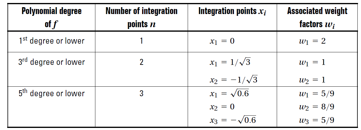
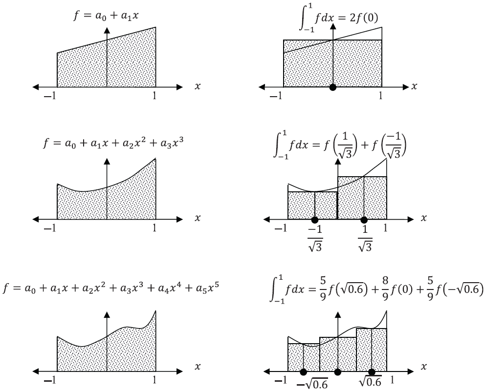
and  is a weight factor associated with each . are termed the integration points. The number of integration points required to obtain sufficient accuracy depends on the shape or form of the function . If is a linear function, then one integration point is enough to exactly integrate . If is a cubic polynomial function, then two integration points are sufficient to obtain the exact solution. Figure 5 shows a graphical representation of the Gauss numerical integration scheme for integrating polynomials up to the fifth degree. Following is a table of the number of integration points required to obtain the exact solution for a polynomial function f with different polynomial degrees:
Example
Verify that the exact integral of a general cubic polynomial on the interval ![[-1, 1]](https://engcourses-uofa.ca/wp-content/ql-cache/quicklatex.com-6e7c9b377ba9e9097d0ab216180a5330_l3.png "Rendered by QuickLaTeX.com") can be obtained by the two integration points
can be obtained by the two integration points  and
and  with the two weight factors
  .
.
Solution
Let  . The exact integral is equal to:
![\[\int_{-1}^1 fdx = 2a_0 + \frac{2a_2}{3}\]](https://engcourses-uofa.ca/wp-content/ql-cache/quicklatex.com-b604d8d0721e9dd742149485fdb86325_l3.png "Rendered by QuickLaTeX.com")
On the other hand, Gauss integration with two integration points is equal to:
![\[\int_{-1}^1 f dx = w_1(a_0+a_1x_1 + a_2x_1^2 + a_3x_1^3) + w_2(a_0 + a_1x_2 + a_2x_2^2 + a_3x_2^3)\]](https://engcourses-uofa.ca/wp-content/ql-cache/quicklatex.com-831b7caa927bcaee64f84139a275a0cb_l3.png "Rendered by QuickLaTeX.com")
Equating the Gauss integration with the exact solution yields the following four equations:
![\[w_1 + w_2 = 2\]](https://engcourses-uofa.ca/wp-content/ql-cache/quicklatex.com-b864cc96b5e6c1db99ae9a79e192ee63_l3.png "Rendered by QuickLaTeX.com")
![\[w_1x_1 + w_2x_2 = 0\]](https://engcourses-uofa.ca/wp-content/ql-cache/quicklatex.com-871545366f954cf4df88f30982cd4edd_l3.png "Rendered by QuickLaTeX.com")
![\[w_1x_1^2 + w_2x_2^2 = \frac{2}{3}\]](https://engcourses-uofa.ca/wp-content/ql-cache/quicklatex.com-8bfbe5328a07f721f1aebf3345d8322a_l3.png "Rendered by QuickLaTeX.com")
![\[w_1x_1^3 + w_2x_2^3 = 0\]](https://engcourses-uofa.ca/wp-content/ql-cache/quicklatex.com-326ccd94d1a89d04e05ee16dba0d9ad3_l3.png "Rendered by QuickLaTeX.com")
These four equations are obtained by noticing that the exact solution and the Gauss integration solution should be equal given any values for the coefficients  ,
,  ,
,  , and
, and  . The solution to the above four equations yields , , . The Mathematica code to solve the four equations is:
View Mathematica Code
View Python Code
from sympy import *
import sympy as sp
sp.init_printing(use_latex = "mathjax")
x1, x2, w1, w2 = sp.symbols("x_1 x_2 w_1 w_2")
#Sympy has a library for Gauss integration
Eq1 = w1+w2-2
Eq2 = w1*x1**3+w2*x2**3
Eq3 = w1*x1**2+w2*x2**2-2/3
Eq4 = w1*x1+w2*x2
s = solve((Eq1,Eq2,Eq3,Eq4), (x1,x2,w1,w2))
display(s)
Note that this example can be extended to show that Gauss integration in one dimension with  points can exactly integrate a polynomial of order
  .
.
Gauss Integration Over Two Dimensional Domains
Let ![f:[-1,1]\times[-1,1]\rightarrow \mathbb{R}](https://engcourses-uofa.ca/wp-content/ql-cache/quicklatex.com-734f55e01d7a646db581496c3fb2073d_l3.png "Rendered by QuickLaTeX.com") . Then, the integral of over the domain can be approximated by the following formula:
. Then, the integral of over the domain can be approximated by the following formula:
![\[\int_{-1}^1 \int_{-1}^1 fdxdy = \sum_{j=1}^n \sum_{i=1}^n w_iw_j f(x_i,y_J)\]](https://engcourses-uofa.ca/wp-content/ql-cache/quicklatex.com-f70100c506af930e7fce6b30be01638e_l3.png "Rendered by QuickLaTeX.com")
where  is an integration point while and
  are weight factors associated with and
  respectively. It can be easily seen that this is a direct consequence of the one dimensional Gauss integration formula as follows:
![\[\int_{-1}^1 \int_{-1}^1 fdxdy = \int_{-1}^1 \sum_{i=1}^n w_i f(x_i,y)dy == \sum_{j=1}^n \sum_{i=1}^n w_iw_j f(x_i,y_J)\]](https://engcourses-uofa.ca/wp-content/ql-cache/quicklatex.com-ef19ac630948edcdc431f85d1bc5422f_l3.png "Rendered by QuickLaTeX.com")
Gauss Integration for Two Dimensional Quadrilateral Isoparametric Elements
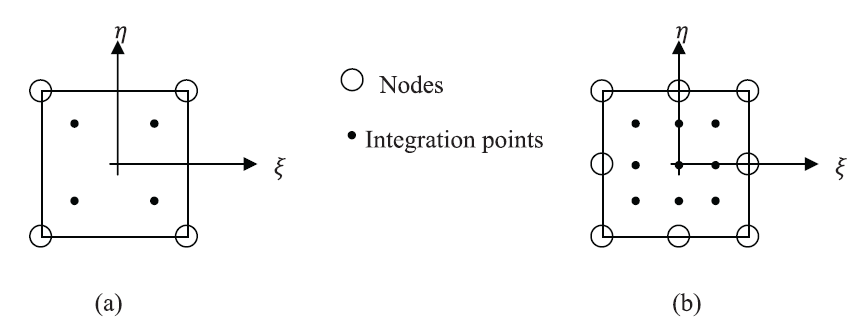
As described for the two dimensional linear quadrilateral element, the strains of the 4 node elements are linear, and thus, the entries in the matrix  are quadratic functions of position. Thus, a
  numerical integration scheme is required to produce accurate integrals for the isoparametric 4-node elements (Figure 6). On the other hand, the strains in the two dimensional quadratic quadrilateral are quadratic functions of position, and thus, the entries in the matrix are fourth-order polynomials of position. Thus, a
  numerical integration scheme is required to produce accurate integrals for the 8 node isoparametric element (Figure 6). It should be noted that this can extended the three dimensional case in a straightforward manner. The 8 node brick element has 8 integration points, while the 20 node brick element has 27 integration points.
 ,
, ,
, with the weight factors
  (b) 8 node isoparametric elements ,
 with the weight factors of
  ,
, , associated with the coordinates
  respectively.
Reduced Gauss Integration (Under Integration) for Two Dimensional Quadilateral Isoparametric Elements
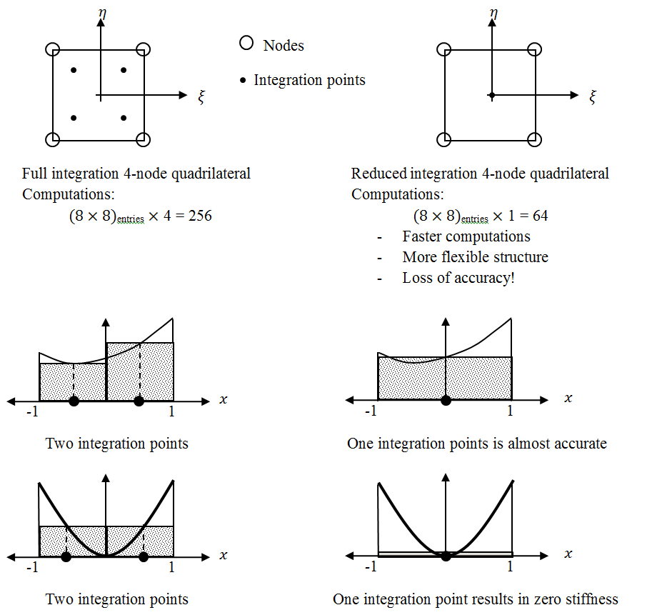
Elements that are integrated as per the previous section are termed “full integration” elements. For example, to integrate the  stiffness matrix of the 4-node plane isoparametric quadrilateral element, each entry will be evaluated at the four locations () of the integration points in the isoparametric element. Thus, the number of computations (excluding the addition) for the integration of the element are
  computations. The number of computations for the
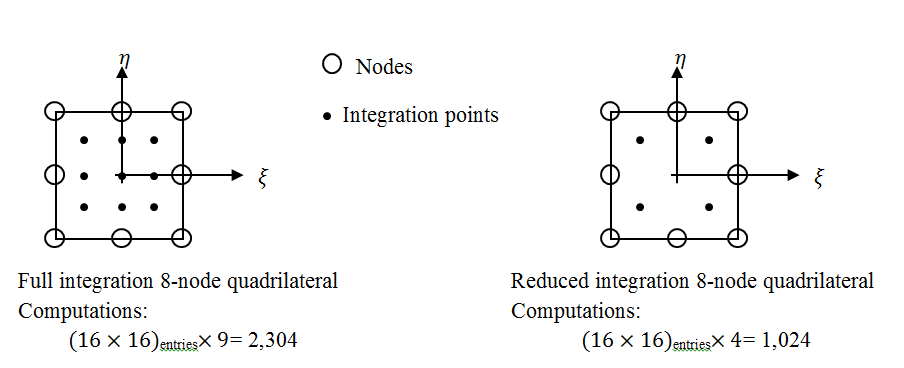
  stiffness matrix of the 8-node plane isoparametric quadrilateral element is 2,304 computations since it uses a
  Gauss integration points scheme! To save computational resources, a “reduced integration” option for each of those elements is available in finite element analysis software. The reduced integration version of the 4-node plane isoparametric quadrilateral element uses only one integration point in the center of the element (Figure 7), and the number of computations is reduced from 256 to 64 computations. However, this is accompanied by a reduction in accuracy. Figure 7 shows two nonlinear functions to be integrated using one integration point vs. two integration points. In the first case, the function has a small variation along the domain and the integration seems to be accurate. However, in the second case, the function has a large variation and is equal to zero in the centre of the domain. The reduced integration will predict zero stiffness!
For the 8-node plane isoparametric quadrilateral, a  Gauss integration points scheme is used instead of the Gauss integration points scheme, which reduces the number of computations from 2,304 to 1,024 computations (Figure 8). The benefit of using reduced integration is not only in saving computational resources but also in balancing out the over-stiffness introduced by assuming a certain deformation field within an element. In fact, reduced integration can lead to better performance in most cases. However, while reduced integration can dramatically reduce the computational time, it can lead to a structure that is too flexible. In fact, the displacements are over predicted when a structure is discretized using reduced integration elements. The reason, as will be shown in the following section, is because some information is lost during sampling of the stiffness at the fewer integration points of the reduced integration elements.
Spurious Modes Associated with Reduced Integration Elements
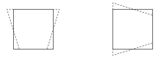
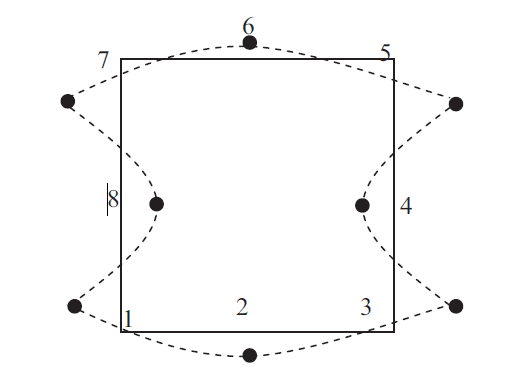
Spurious modes, or sometimes called zero energy modes, are combinations of displacements that in general produce strains; however, such strains cannot be detected at the integration or sampling points. So, the internal energy calculated at the integration points is equal to zero for such mode. In other words, a very small amount of load would be enough to produce a very large displacement. If a spurious mode exists for the whole structure, it becomes unstable. Usually spurious modes exist in under-integrated element (reduced integration). This is because the reduced number of integration points cannot detect a spurious strain mode. The two very common spurious modes are those for the bilinear quadrilateral (4-node plane element) and the quadratic displacement quadrilateral (8-node plane element). In general, any bending mode is a spurious mode in a 4-node reduced-integration linear element. The strain modes shown cannot be detected at the integration point; the strain at the center of the element (at the location of the single integration point) is equal to zero (Figure 9). On the other hand, the spurious mode of an 8 node reduced integration quadratic element is called “the hour glass” mode (Figure 10) and is produced with the following configuration of nodal displacements:
![\[u_1 = u_7 = v_5 = v_7 = 1 \hspace{5mm} u_3 = u_5 = v_1 = v_3 = 1 \hspace{5mm} v_6 = u_8 = \frac{1}{2} = -u_4 = -v_2\]](https://engcourses-uofa.ca/wp-content/ql-cache/quicklatex.com-0d0b271905bc6e415ec3d53f6a7527ed_l3.png "Rendered by QuickLaTeX.com")
The spurious modes will be illustrated using the following problem.
Example
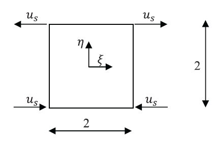
Find the internal energy associated with the shown displacement for the 4-node plane stress quadrilateral element shown below, assuming a bilinear displacement interpolation function.
Use exact integration, full integration ( integration points), and reduced integration (1 integration point).
Solution
The shape functions of the shown element are:
![\[N_1 = \frac{(1-\xi)(1-\eta)}{4}\]](https://engcourses-uofa.ca/wp-content/ql-cache/quicklatex.com-7dd29e33b3ee0e9a3086f78f575a29eb_l3.png "Rendered by QuickLaTeX.com")
![\[N_2 = \frac{(1+\xi)(1-\eta)}{4}\]](https://engcourses-uofa.ca/wp-content/ql-cache/quicklatex.com-7762cfc1e0306958b16f40631faa0d92_l3.png "Rendered by QuickLaTeX.com")
![\[N_3 = \frac{(1+\xi)(1+\eta)}{4}\]](https://engcourses-uofa.ca/wp-content/ql-cache/quicklatex.com-002cc5aeb41b2aced47c5a631aa02f16_l3.png "Rendered by QuickLaTeX.com")
![\[N_4 = \frac{(1-\xi)(1+\eta)}{4}\]](https://engcourses-uofa.ca/wp-content/ql-cache/quicklatex.com-4a7dda36801b74d10ce5f45c257e5307_l3.png "Rendered by QuickLaTeX.com")
The displacement functions  and
and  in the directions and
  , respectively, are:
![\[u = u_sN_1 - u_sN_2 + u_sN_3 - u_sN_4 \hspace{5mm} v = 0\]](https://engcourses-uofa.ca/wp-content/ql-cache/quicklatex.com-ca684a08ab202d759b02050b696ce74d_l3.png "Rendered by QuickLaTeX.com")
Therefore, the strains have the form:
![\[\begin{pmatrix} \varepsilon_{\xi \xi} \\ \varepsilon_{\eta \eta} \\ \gamma_{\xi \eta} \\ \end{pmatrix} = \begin{pmatrix} \frac{\partial N_1}{\partial \xi} -\frac{\partial N_2}{\partial \xi} + \frac{\partial N_3}{\partial \xi} - \frac{\partial N_3}{\partial \xi} \\ 0 \\ \frac{\partial N_1}{\partial \eta} - \frac{\partial N_2}{\partial \eta} + \frac{\partial N_3}{\partial \eta} - \frac{\partial N_4}{\partial \eta} \\ \end{pmatrix} u_s = Bu_s\]](https://engcourses-uofa.ca/wp-content/ql-cache/quicklatex.com-c421c924980daad8a1f0ea74e40dc0d5_l3.png "Rendered by QuickLaTeX.com")
The stress strain relationship for plane stress is given by:
![\[\begin{pmatrix} \sigma_{\xi \xi} \\ \sigma_{\eta \eta} \\ \sigma_{\xi \eta} \\ \end{pmatrix} = \frac{E}{(1+\nu)(1-\nu)} \begin{pmatrix} 1 & \nu & 0 \\ \nu & 1 & 0 \\ 0 & 0 & \frac{(1-\nu)}{2} \\ \end{pmatrix} \begin{pmatrix} \varepsilon_{\xi \xi} \\ \varepsilon_{\eta \eta} \\ \gamma_{\xi \eta} \\ \end{pmatrix}\]](https://engcourses-uofa.ca/wp-content/ql-cache/quicklatex.com-99eccbc04b99d26d1424ca8f4982149e_l3.png "Rendered by QuickLaTeX.com")
The stiffness matrix  can be evaluated using the following integral where
  is the element thickness:
![\[K = t \int_{-1}^1 \int_{-1}^1 B^T CB d\xi d\eta = \frac{tE}{2(\nu^2-1)} \int_{-1}^1 \int_{-1}^1 (\nu-1)\xi^2 - 2\eta^2 d\xi d\eta\]](https://engcourses-uofa.ca/wp-content/ql-cache/quicklatex.com-15d0460dbf1a9e73ed38787f0abec751_l3.png "Rendered by QuickLaTeX.com")
Notice that the system has only one degree of freedom (the unknown displacement variable  ), and therefore, the stiffness matrix has the dimensions
  .
.
Using Exact Integration:
The stiffness matrix evaluated using exact integration is:
![\[K = \frac{2E(\nu-3)}{3(\nu^2-1)}\]](https://engcourses-uofa.ca/wp-content/ql-cache/quicklatex.com-5a63aeb2a9755f7a0212565760338790_l3.png "Rendered by QuickLaTeX.com")
The strain energy associated with this displacement mode is equal to:
![\[\frac{1}{2}Ku_s^2 = \frac{2E(\nu-3)}{6(\nu^2-1)} u_s^2\]](https://engcourses-uofa.ca/wp-content/ql-cache/quicklatex.com-c254ad69c4f73cb7f36f156dfb143456_l3.png "Rendered by QuickLaTeX.com")
Using Full Integration:
The stiffness matrix evaluated using full integration is:
![\[K = \frac{tE}{2(\nu^2-1)} \Big(\sum_{i,j=1}^2 w_iw_j ((\nu-1)\xi_i^2 - 2\eta_j^2) \Big) = \frac{2E(\nu-3)}{3(\nu^2-1)}\]](https://engcourses-uofa.ca/wp-content/ql-cache/quicklatex.com-d9d0d953cb82d6e77562145e7242941b_l3.png "Rendered by QuickLaTeX.com")
where  and which gives the same results as the exact integration.
Using Reduced Integration:
The stiffness matrix evaluated using reduced integration is:
![\[K = \frac{tE}{2(\nu^2-1)} \Big(\sum_{i,j=1}^1 w_iw_j ((\nu-1)\xi_i^2 - 2\eta_j^2) \Big) = 0\]](https://engcourses-uofa.ca/wp-content/ql-cache/quicklatex.com-ad275ad763221ad390acd5fa6fcecf3b_l3.png "Rendered by QuickLaTeX.com")
where  and
and  . The strain energy associated with this displacement mode is equal to zero. Thus, the reduced integration scheme predicts that the displacement field shown does not require any external forces applied to the element. Thus, this element is unstable if loads produce the displacement mode shown, i.e., bending! The following is the Mathematica code used for the above calculations:
View Mathematica Code
N1=(1-xi)(1-eta)/4;
N2=(1+xi)(1-eta)/4;
N3=(1+xi)(1+eta)/4;
N4=(1-xi)(1+eta)/4;
B={D[N1-N2+N3-N4,xi],0,D[N1-N2+N3-N4,eta]};
Cc=Ee/(1+nu)/(1-nu)*{{1,nu,0},{nu,1,0},{0,0,(1-nu)/2}};
Kbeforeintegration=FullSimplify[B.Cc.B]
(*Using Exact Integration*)
Kexact=Integrate[Kbeforeintegration,{eta,-1,1},{xi,-1,1}]
Energyexact=us*Kexact*us/2
(*Using Full Integration*)
etaset={1/Sqrt[3],-1/Sqrt[3]};
xiset={1/Sqrt[3],-1/Sqrt[3]};
Kfull=FullSimplify[Sum[(Kbeforeintegration/.{xi->xiset[[i]],eta->etaset[[j]]}),{i,1,2},{j,1,2}]]
Energyfull=us*Kfull*us/2
(*Using reduced Integration*)
etaset=xiset={0};
Kreduced=Sum[4(Kbeforeintegration/.{xi->xiset[[i]],eta->etaset[[j]]}),{i,1,1},{j,1,1}]
Energyreduced=us*Kreduced*us/2
View Python Code
from sympy import *
import sympy as sp
sp.init_printing(use_latex = "mathjax")
xi, eta, nu, E, us = sp.symbols("xi eta nu E u_s")
N1=(1-xi)*(1-eta)/4
N2=(1+xi)*(1-eta)/4
N3=(1+xi)*(1+eta)/4
N4=(1-xi)*(1+eta)/4
B = Matrix([(N1-N2+N3-N4).diff(xi),0,(N1-N2+N3-N4).diff(eta)])
Cc = E/(1+nu)/(1-nu)*Matrix([[1,nu,0],[nu,1,0],[0,0,(1-nu)/2]])
display(B,Cc)
KBeforeintegration = simplify(B.transpose()*Cc*B)
display("K before integration: ", KBeforeintegration)
display("Using Exact Integration")
etaset = Matrix([1/sqrt(3), -1/sqrt(3)])
xiset = Matrix([1/sqrt(3), -1/sqrt(3)])
Kfull = 0
for i in range(2):
    for j in range(2):
        Kfull += KBeforeintegration[0].subs({xi:xiset[i], eta:etaset[j]})
display(simplify(Kfull))
Energyfull = us*Kfull*us/2
display(simplify(Energyfull))
display("Using reduced integration")
etaset = xiset = Matrix([0])
Kreduced = 4*KBeforeintegration[0].subs({xi:xiset[0], eta:etaset[0]})
display(Kreduced)
Energyreduced=us*Kreduced*us/2
Gauss Integration for Two Dimensional Triangle Isoparametric Elements
The strains of the 3 node triangle element are constant, and thus, the entries in the matrix are constant. Thus, a 1 point numerical integration scheme is required to produce accurate integrals for the isoparametric 3-node elements (Figure 11). For the 6 node triangle element, a 3 points numerical integration scheme is required to produce accurate integrals (Figure 11). It should be noted that the shown locations for the integration points and their number can be extended to the three-dimensional case in a straightforward manner.
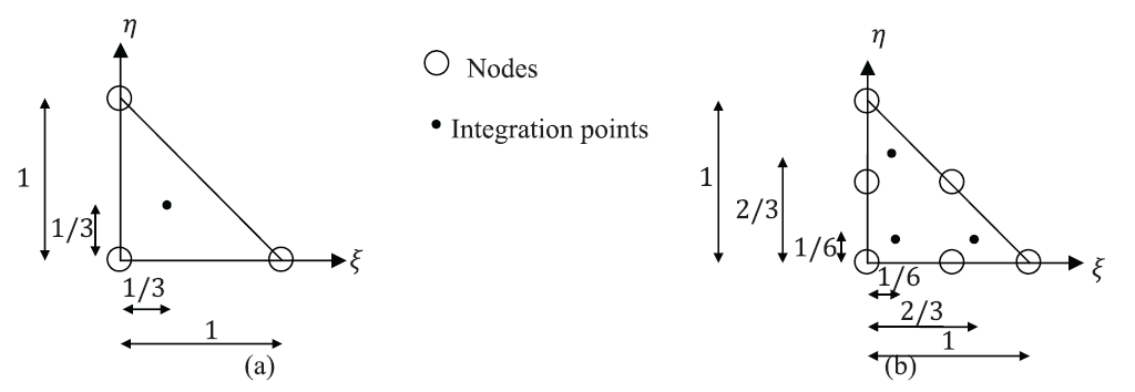
 and
and  . (b) 6 node isoparametric elements
  with equal weight factors
  .
.Final Notes
The use of isoparametric elements and numerical integration dramatically increases the robustness of the finite element analysis method. The techniques described in the previous sections allow meshing of irregular domains with compatible elements, i.e., elements that ensure the continuity of the displacement field across boundaries (How?). However, to ensure the continuity of the displacement field, the elements of the mesh should be of the same type; otherwise, the user has to apply mesh constraints to ensure the compatibility of the displacement between elements. For example, a 4-node bilinear displacement element when connected to an 8-node quadratic displacement element will have incompatible displacements at the side of the connection. This can be overcome by constraining the mid-side node of the quadratic element to always lie on the straight side of the bilinear element. Otherwise, the results at the location of discontinuous displacement fields would be erroneous.
The stiffness matrix and the nodal loads of the structure can be calculated using the Gauss numerical integration scheme, which speeds up the computational time required. However, the price of using the Gauss numerical integration is the loss of accuracy. Gauss numerical integration produces accurate results only when the integrals are exact polynomials. The integrals are exact polynomials only when the elements of the mesh are exactly aligned with the isoparametric mapping into the coordinates of and . When the shape of the elements in the mesh deviates from the shape of the element in the coordinate system of and , the functions to be integrated are no longer exact polynomials but rather radicals; thus, the numerical integration scheme is no longer accurate. Most finite element analysis software give warnings when elements are highly distorted since this will lead to inaccurate computations of the stiffness matrix during the numerical integration process. In addition, for nonlinear problems when the stiffness changes with deformation, it is possible that the element will reach a highly distorted shape that the numerical integration scheme is no longer valid.