
Plane Beam Approximations: Examples and Problems
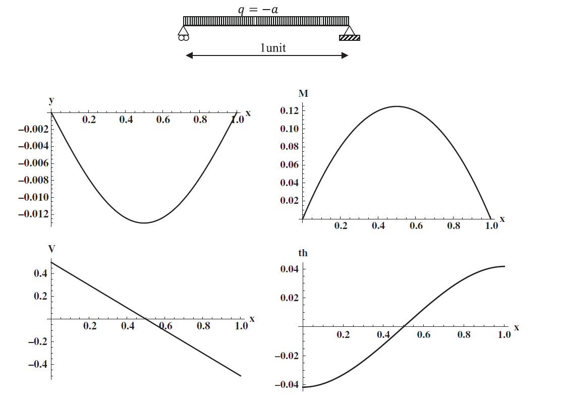
Example 1: Euler Bernoulli Simple Beam
Find the deflection, rotation, bending moment, and shearing force as a function of the beam length of an Euler Bernoulli simple beam assuming  units,
  units and
  unit.
unit.
Solution
The DSolve function in Mathematica is used to solve the differential equation of equilibrium with four boundary conditions  and
and  on both the left and right ends of the beam.
View Mathematica Code
Clear[a,x,V,M,y,L,EI]
M=EI*D[y[x],{x,2}];
V=EI*D[y[x],{x,3}];
th=D[y[x],x];
q=-a;
M1=M/.x->0;
M2=M/.x->L;
V1=V/.x->0;
V2=V/.x->L;
y1=y[x]/.x->0;
y2=y[x]/.x->L;
th1=th/.x->0;
th2=th/.x->L;
s=DSolve[{EI*y''''[x]==q,M1==0,M2==0,y1==0,y2==0},y,x];
y=y[x]/.s[[1]];
th=D[y,x];
M=EI*D[y,{x,2}];
V=EI*D[y,{x,3}];
y/.x->L/2
EI=1;
a=1;
L=1;
Plot[y,{x,0,L},BaseStyle->Directive[Bold,15],PlotRange->All,AxesLabel->{"x","y"},PlotStyle->{Black,Thickness[0.005]}]
Plot[M,{x,0,L},PlotRange->All,BaseStyle->Directive[Bold,15],AxesLabel->{"x","M"},PlotStyle->{Black,Thickness[0.005]}]
Plot[V,{x,0,L},BaseStyle->Directive[Bold,15],PlotRange->All,AxesLabel->{"x","V"},PlotStyle->{Black,Thickness[0.005]}]
Plot[th,{x,0,L},PlotRange->All,BaseStyle->Directive[Bold,15],AxesLabel->{"x","th"},PlotStyle->{Black,Thickness[0.005]}]
View Python Code
from sympy import *
from numpy import *
import sympy as sp
import numpy as np
import matplotlib.pyplot as plt
sp.init_printing(use_latex = "mathjax")
a, L, x , EI = symbols("a L x EI")
q = -a
fig, ax = plt.subplots(2,2, figsize = (10,6))
plt.setp(ax[0,0], xlabel = "x", ylabel = "y")
plt.setp(ax[0,1], xlabel = "x", ylabel = "M")
plt.setp(ax[1,1], xlabel = "x", ylabel = "th")
plt.setp(ax[1,0], xlabel = "x", ylabel = "V")
y = Function("y")
th = y(x).diff(x)
M = EI * y(x).diff(x,2)
V = EI * y(x).diff(x,3)
M1 = M.subs(x,0)
M2 = M.subs(x,L)
V1 = V.subs(x,0)
V2 = V.subs(x,L)
y1 = y(x).subs(x,0)
y2 = y(x).subs(x,L)
s = dsolve(EI*y(x).diff(x,4)-q, y(x),ics={M1/EI:0,M2/EI:0,y1:0,y2:0})
y = s.rhs
th = y.diff(x)
M = EI * y.diff(x,2)
V = EI * y.diff(x,3)
x1 = np.arange(0,1.1,0.1)
y = y.subs({L:1, a:1, EI:1})
y_list = [y.subs({x:i}) for i in x1]
th = th.subs({L:1, a:1, EI:1})
th_list = [th.subs({x:i}) for i in x1]
M = M.subs({L:1, a:1, EI:1})
M_list = [M.subs({x:i}) for i in x1]
V = V.subs({L:1, a:1, EI:1})
V_list = [V.subs({x:i}) for i in x1]
ax[0,0].plot(x1, y_list)
ax[0,1].plot(x1, M_list)
ax[1,0].plot(x1, V_list)
ax[1,1].plot(x1, th_list)
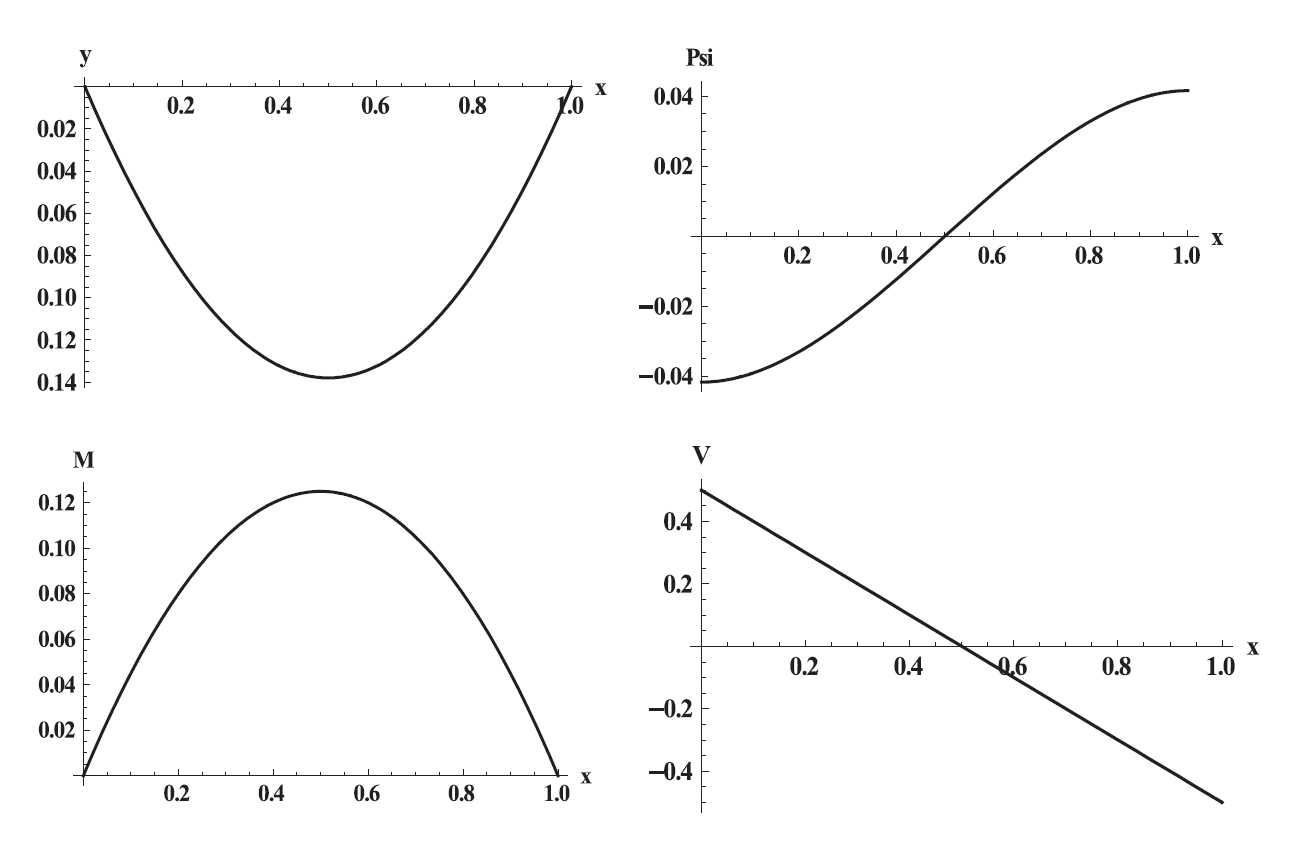
Example 2: Timoshenko Simple Beam
Find the deflection, rotation, bending moment, and shearing force as a function of the beam length of a Timoshenko simple beam assuming units, units,  unit and unit.
SOLUTION
The DSolve function in Mathematica is used to solve the differential equation of equilibrium with four boundary conditions and on both the left and right ends of the beam.
View Mathematica Code
Clear[a, x, V, M, y, L, psi, EI, kAG]
M = EI*D[psi[x], x];
V = EI*D[psi[x], {x, 2}];
q = -a;
M1 = M /. x -> 0;
M2 = M /. x -> L;
V1 = V /. x -> 0;
V2 = V /. x -> L;
y1 = y[x] /. x -> 0;
y2 = y[x] /. x -> L;
psi1 = psi[x] /. x -> 0;
psi2 = psi[x] /. x -> L;
s = DSolve[{EI*psi'''[x] == q, psi[x] == y'[x] + EI/kAG*psi''[x],
    M1 == 0, M2 == 0, y1 == 0, y2 == 0}, {y, psi}, x];
y = y /. s[[1, 2]];
psi = psi /. s[[1, 1]];
y[L/2]
EI = 1;
a = 1;
L = 1;
kAG = 1;
Plot[y[x], {x, 0, L}, BaseStyle -> Directive[Bold, 15],
 PlotRange -> All, AxesLabel -> {"x", "y"},
 PlotStyle -> {Black, Thickness[0.005]}]
Plot[psi[x], {x, 0, L}, PlotRange -> All,
 BaseStyle -> Directive[Bold, 15], AxesLabel -> {"x", "Psi"},
 PlotStyle -> {Black, Thickness[0.005]}]
Plot[M, {x, 0, L}, PlotRange -> All, BaseStyle -> Directive[Bold, 15],
  AxesLabel -> {"x", "M"}, PlotStyle -> {Black, Thickness[0.005]}]
Plot[V, {x, 0, L}, PlotRange -> All, BaseStyle -> Directive[Bold, 15],
  AxesLabel -> {"x", "V"}, PlotStyle -> {Black, Thickness[0.005]}]
View Python Code
from sympy import *
from numpy import *
import sympy as sp
import numpy as np
import matplotlib.pyplot as plt
sp.init_printing(use_latex = "mathjax")
a, L, x , EI, psi, kAG, C1, C2, C3, C4 = symbols("a L x EI psi kAG C_1 C_2 C_3 C_4")
q = -a
fig, ax = plt.subplots(2,2, figsize = (10,6))
plt.setp(ax[0,0], xlabel = "x", ylabel = "y")
plt.setp(ax[0,1], xlabel = "x", ylabel = "Psi")
plt.setp(ax[1,0], xlabel = "x", ylabel = "M")
plt.setp(ax[1,1], xlabel = "x", ylabel = "V")

# With general integration
EIpsi = integrate(q,x,x,x) + C1*x**2/2 + C2*x + C3
display(EIpsi)
EIy = integrate(q,x,x,x,x) + C1*x**3/6 + C2*x**2/2 + C3*x + C4 - EI/kAG*(integrate(q,x,x) + C1*x)
display(EIy)
M = EIpsi.diff(x)
V = EIpsi.diff(x,2)
display(M,V)
M1 = M.subs(x,0)
M2 = M.subs(x,L)
y1 = (EIy/EI).subs(x,0)
y2 = (EIy/EI).subs(x,L)
display(M1,M2,y1,y2)
s = solve([M1,M2,y1,y2], [C1, C2, C3, C4])
display(s)
x1 = np.arange(0,1.1,0.1)
EIpsi = EIpsi.subs({C1:s[C1], C2:s[C2], C3:s[C3], C4:s[C4], a:1, L:1, kAG:1, EI:1})
psi_list = [EIpsi.subs({x:i}) for i in x1]
display(EIpsi)
EIy = EIy.subs({C1:s[C1], C2:s[C2], C3:s[C3], C4:s[C4], a:1, L:1, kAG:1, EI:1})
y_list = [EIy.subs({x:i}) for i in x1]
display(EIy)
M = M.subs({C1:s[C1], C2:s[C2], C3:s[C3], a:1, L:1, kAG:1, EI:1})
M_list = [M.subs({x:i}) for i in x1]
display(M)
V = V.subs({C1:s[C1], C2:s[C2], C3:s[C3], a:1, L:1, kAG:1, EI:1})
V_list = [V.subs({x:i}) for i in x1]
display(V)
ax[0,0].plot(x1, y_list)
ax[0,1].plot(x1, psi_list)
ax[1,0].plot(x1, M_list)
ax[1,1].plot(x1, V_list)
Example 3: Bending and Shear Stresses in an Euler Brnoulli Cantilever Beam
Consider a cantilever Euler Bernoulli beam with Young’s modulus  . The beam is 5m long and has a rectangular cross section. The height of the beam is 0.5m, while the width is 0.25m.
If a load of 125kN is applied downwards at the free end, draw the contour plot of  ,
,  ,
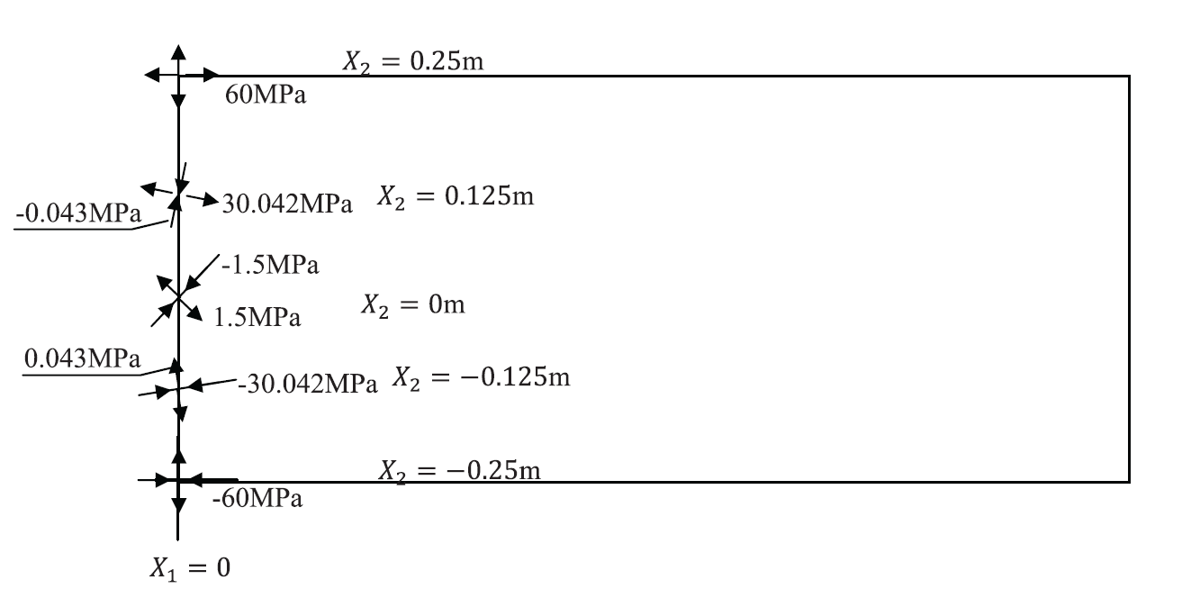
,  along the beam. Also, sketch the principal stress directions at the top fibers, the bottom fibers, the neutral axis and at quarter of the height of the beam at the support
  . Also, draw the vector plot of the displacement of the beam.
SOLUTION
The first step is to solve for the beam deflection by solving the differential equation of equilibrium with  :
:
![\[EI\frac{\mathrm{d}^4y}{\mathrm{d}X_1^4}=q=0\Rightarrow y=C_1\frac{X_1^3}{6}+C_2\frac{X_1^2}{2}+C_3X_1+C_4\]](https://engcourses-uofa.ca/wp-content/ql-cache/quicklatex.com-7a4a0ead4edda3b8aa3e83c9f2ac1e73_l3.png "Rendered by QuickLaTeX.com")
where  is the moment of inertia and
  and
and  are given. The constants
  can be solved using the boundary conditions:
![\[\begin{split}@X_1=0 & :y=0\\@X_1=0 & :\theta=\frac{\mathrm{d}y}{\mathrm{d}X_1}=0\\@X_1=5 & :V=EI\frac{\mathrm{d}^3y}{\mathrm{d}X_1^3}=125\\@X_1=5 & :M=EI\frac{\mathrm{d}^2y}{\mathrm{d}X_1^2}=0\end{split}\]](https://engcourses-uofa.ca/wp-content/ql-cache/quicklatex.com-7fe0d9bd543d033b7d3a10bc35aa658b_l3.png "Rendered by QuickLaTeX.com")
Therefore, the displacement function  is:
is:
![\[y=\frac{-125}{6EI}(3LX_1^2-X_1^3)\]](https://engcourses-uofa.ca/wp-content/ql-cache/quicklatex.com-daaf58a121e9484a3499ef868696eb16_l3.png "Rendered by QuickLaTeX.com")
From which the moment and the shear can be obtained as:
![\[M=EI\frac{\mathrm{d}^2y}{\mathrm{d}X_1^2}=125(X_1-5) kN.m.\qquad V=EI\frac{\mathrm{d}^3y}{\mathrm{d}X_1^3}=125 kN\]](https://engcourses-uofa.ca/wp-content/ql-cache/quicklatex.com-0fbecbf3dd9e26ee95eae8cd786dff43_l3.png "Rendered by QuickLaTeX.com")
The stresses along the beam length and depth can be obtained as functions of  and
and  as follows:
![\[\sigma_{11}=\frac{-MX_2}{I}=-\frac{125(X_1-5)X_2}{I}\qquad \sigma_{12}=\frac{-VQ}{Ib}=-\frac{125\left(\frac{t}{2}-X_2\right)\left(\frac{X_2}{2}+\frac{t}{4}\right)}{I}\]](https://engcourses-uofa.ca/wp-content/ql-cache/quicklatex.com-1d8f2edb13b7f220a3c598f12bf400a9_l3.png "Rendered by QuickLaTeX.com")
the vector of displacement of the beam is given by:
![\[u=x-X=\left(\begin{array}{c}-X_2\frac{\mathrm{d}y}{\mathrm{d}X_1}\\y\\0\end{array}\right)\]](https://engcourses-uofa.ca/wp-content/ql-cache/quicklatex.com-085596552f3fd483fe5160ab9d30f2e0_l3.png "Rendered by QuickLaTeX.com")
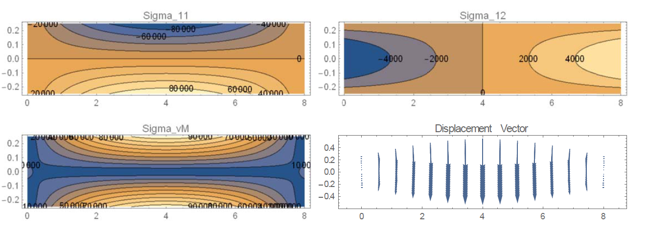
The required plots are shown below.
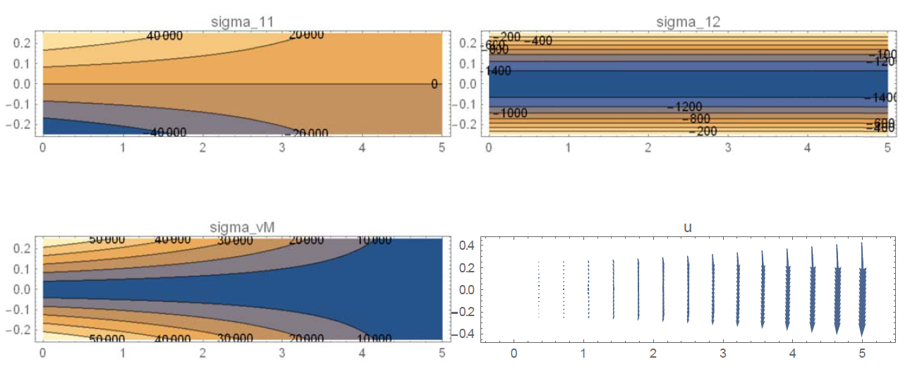
As shown in the plots, the bending stress is positive at the top (tension) and negative at the bottom, and increases in magnitude towards the support. The shearing stress component is constant at the neutral axis (Why?) throughout the length of the beam and decreases toward zero at the top and bottom fibers of the beam. The von Mises stress distribution follows the bending stress component, but gives a positive value in tension and in compression!
The eigenvalues and the eigenvectors of the stress matrix at the specified locations are obtained using Mathematica and are sketched below. The shear stresses at the top and bottom fibers are zero, and thus, the principal stresses are aligned with the chosen orthonormal coordinate system. At the location of the neutral axis of the beam, the bending stress component is zero, and the only nonzero component is , thus, the principal stresses at the neutral axis are aligned at 45 degrees. The direction of the principal stress with the highest magnitude at  is along the vector {0.9993, –0.0374212,0}. At
  , the principal stress with magnitude –30.042MPa is aligned with the vector {0.9993,0.0374212,0}.
View Mathematica Code
Clear[a,x,V,M,y,L,EI]
M=EI*D[y[x],{x,2}];
V=EI*D[y[x],{x,3}];
th=D[y[x],x];
M1=M/.x->0;
M2=M/.x->L;
V1=V/.x->0;
V2=V/.x->L;
y1=y[x]/.x->0;
y2=y[x]/.x->L;
th1=th/.x->0;
th2=th/.x->L;
s=DSolve[{EI*y''''[x]==0,M2==0,V2==125,y1==0,th1==0},y,x]
y=y[x]/.s[[1]]
EI=Ee*Ii;
u = {X2*-D[y, x], y}
M=FullSimplify[M/.s[[1]]]
V=V/.s[[1]]
Ee=20000000;
b=0.25;
t=0.5;
L=5;
Ii=b*t^3/12;
s11=-M*X2/Ii;
Q=(t/2-X2)*b*(t/4+X2/2)
s12=-V*Q/Ii/b;
smatrix={{s11,s12,0},{s12,0,0},{0,0,0}};
FullSimplify[Chop[smatrix]]//MatrixForm
VonMises[sigma_]:=Sqrt[1/2*((sigma[[1,1]]-sigma[[2,2]])^2+(sigma[[2,2]]-sigma[[3,3]])^2+(sigma[[3,3]]-sigma[[1,1]])^2+6*(sigma[[1,2]]^2+sigma[[1,3]]^2+sigma[[2,3]]^2))];
vonmisesstress=VonMises[smatrix]
ContourPlot[s11, {x, 0, 5}, {X2, -0.25, 0.25}, AspectRatio -> 0.25, ContourLabels -> True, PlotLabel -> "sigma_11"]
ContourPlot[s12, {x, 0, 5}, {X2, -0.25, 0.25}, AspectRatio -> 0.25, ContourLabels -> True, PlotLabel -> "sigma_12"]
ContourPlot[vonmisesstress, {x, 0, 5}, {X2, -0.25, 0.25}, AspectRatio -> 0.25, ContourLabels -> True, PlotLabel -> "sigma_vM"]
VectorPlot[u, {x, 0, 5}, {X2, -0.25, 0.25}, AspectRatio -> 0.25, PlotLabel -> "u"]
stressmat1=smatrix/.{x->0,X2->-0.25}
Eigensystem[stressmat1]
stressmat2=smatrix/.{x->0,X2->-0.25/2}
Eigensystem[stressmat2]
stressmat3=smatrix/.{x->0,X2->0}
Eigensystem[stressmat3]
stressmat4=smatrix/.{x->0,X2->0.25/2}
Eigensystem[stressmat4]
stressmat5=smatrix/.{x->0,X2->0.25}
Eigensystem[stressmat5]
stressmat1=smatrix/.{x->1,X2->-0.25}
Eigensystem[stressmat1]
stressmat2=smatrix/.{x->1,X2->-0.25/2}
Eigensystem[stressmat2]
stressmat3=smatrix/.{x->1,X2->0}
Eigensystem[stressmat3]
stressmat4=smatrix/.{x->1,X2->0.25/2}
Eigensystem[stressmat4]
stressmat5=smatrix/.{x->1,X2->0.25}
Eigensystem[stressmat5]
View Python Code
from sympy import *
from numpy import *
import sympy as sp
import numpy as np
import matplotlib.pyplot as plt
sp.init_printing(use_latex = "mathjax")
x , EI, X2, L, I, t, E= symbols("x EI X_2 L I t Ee")

def vonMises(M):
    return sp.sqrt(1/2*((M[0,0] - M[1,1])**2+(M[1,1] - M[2,2])**2+
                       (M[2,2] - M[0,0])**2+6*(M[0,1]**2+M[0,2]**2+M[1,2]**2)))

def plotContour(f, limits, title):
    x1, xn, y1, yn = limits
    dx, dy = 10/100*(xn-x1),10/100*(yn - y1)
    xrange = np.arange(x1,xn+dx,dx)
    yrange = np.arange(y1,yn+dy,dy)
    X, Y = np.meshgrid(xrange, yrange)
    lx, ly = len(xrange), len(yrange)
    F = lambdify((x,X2),f)
    # if F is constant, then generates array
    # if F generates array, doesn't change anything
    Z = F(X,Y)*np.ones(lx*ly).reshape(lx, ly)
    fig = plt.figure(figsize = (8,2))
    ax = fig.add_subplot(111)
    cp = ax.contourf(X,Y,Z)
    fig.colorbar(cp)
    plt.title(title)

def plotVector(f, limits, title):
    fx, fy = [lambdify((x,X2),fi) for fi in f]
    x1, xn, y1, yn = limits
    dx, dy = 10/100*(xn-x1),10/100*(yn-y1)
    xrange = np.arange(x1,xn,dx)
    yrange = np.arange(y1,yn,dy)
    X, Y = np.meshgrid(xrange, yrange)
    dxplot, dyplot = fx(X,Y), fy(X,Y)
    fig = plt.figure(figsize = (7.5,2))
    ax = fig.add_subplot(111)
    ax.quiver(X, Y, dxplot, dyplot)
    plt.title(title)

y = Function('y')
th = y(x).diff(x)
M = EI * y(x).diff(x,2)
V = EI * y(x).diff(x,3)
M1 = M.subs(x,0)
M2 = M.subs(x,L)
V1 = V.subs(x,0)
V2 = V.subs(x,L)
y1 = y(x).subs(x,0)
y2 = y(x).subs(x,L)
th1 = th.subs(x,0)
th2 = th.subs(x,L)
s = dsolve(EI*y(x).diff(x,4), y(x), ics = {M2/EI:0,V2/EI:125/EI,y1:0, th1:0})
display("displacement function: ",s)
y = s.rhs
u = Matrix([[X2* -y.diff(x)], [y]])
M = EI * y.diff(x,2)
V = EI * y.diff(x,3)
display("Moment: ", M.subs(L,5))
display("Shear: ", V)
s11 = -M*X2/I
b = 0.25
Q = (t/2 - X2) * b * (t/4 + X2/2)
s12 = -V * Q/I/b
display("stresses: ", s11, s12)
s11 = s11.subs({E:20000000, t:0.5, L:5, I:b*t**3/12})
s12 = s12.subs({E:20000000, t:0.5, L:5, I:b*t**3/12})
smatrix = Matrix([[s11, s12, 0], [s12, 0, 0], [0, 0, 0]])
vonMisesstress = vonMises(smatrix)
display("von Mises stress: ", vonMisesstress)
plotContour(s11, [0,5,-0.25,0.25], "sigma_11")
plotContour(s12, [0,5,-0.25,0.25], "sigma_12")
plotContour(vonMisesstress, [0,5,-0.25,0.25], "sigma_vM")
u = u.subs({E:20000000, t:0.5, L:5, Ii:b*t**3/12, EI:E*Ii})
plotVector(u, [0,5,-0.25,0.25], "u")
stressmat1 = smatrix.subs({x:0, X2: -0.25})
display("stress matrix 1 eigensystem(x = 0, X2 = -0.25): ", stressmat1.eigenvects())
stressmat2 = smatrix.subs({x:0, X2: -0.25/2})
display("stress matrix 2 eigensystem(x = 0, X2 = -0.25/2): ", stressmat2.eigenvects())
stressmat3 = smatrix.subs({x:0, X2: 0})
display("stress matrix 3 eigensystem(x = 0, X2 = 0): ", stressmat3.eigenvects())
stressmat4 = smatrix.subs({x:0, X2: 0.25/2})
display("stress matrix 4 eigensystem(x = 0, X2 = 0.25/2): ", stressmat4.eigenvects())
stressmat5 = smatrix.subs({x:0, X2: 0.25})
display("stress matrix 5 eigensystem(x = 0, X2 = 0.25): ", stressmat5.eigenvects())
stressmat1_2 = smatrix.subs({x:0, X2: -0.25})
display("stress matrix 1 eigensystem(x = 1, X2 = -0.25): ", stressmat1_2.eigenvects())
stressmat2_2 = smatrix.subs({x:1, X2: -0.25/2})
display("stress matrix 2 eigensystem(x = 1, X2 = -0.25/2): ", stressmat2_2.eigenvects())
stressmat3_2 = smatrix.subs({x:1, X2: 0})
display("stress matrix 3 eigensystem(x = 1, X2 = 0): ", stressmat3_2.eigenvects())
stressmat4_2 = smatrix.subs({x:1, X2: 0.25/2})
display("stress matrix 4 eigensystem(x = 1, X2 = 0.25/2): ", stressmat4_2.eigenvects())
stressmat5_2 = smatrix.subs({x:1, X2: 0.25})
display("stress matrix 5 eigensystem(x = 1, X2 = 0.25): ", stressmat5_2.eigenvects())
Example 4: Bending and Shear Stresses in an Euler Bernoulli Simple Beam
Consider an Euler Bernoulli simple beam with Young’s modulus . The beam is 8m long and has a rectangular cross section. The height of the beam is 0.5m, while the width is 0.25m. If a load of 125kN/m is distributed over the beam length, draw the contour plot of , , and along the beam. Also, draw the vector plot of the displacement of the beam.
SOLUTION
The first step is to solve for the beam deflection by solving the differential equation of equilibrium with  :
:
![\[EI\frac{\mathrm{d}^4y}{\mathrm{d}X_1^4}=q=-125\Rightarrow EIy=-125\frac{X_1^4}{24}+C_1\frac{X_1^3}{6}+C_2\frac{X_1^2}{2}+C_3X_1+C_4\]](https://engcourses-uofa.ca/wp-content/ql-cache/quicklatex.com-ec4a1eb482f981319b3baa76895b5b23_l3.png "Rendered by QuickLaTeX.com")
where is the moment of inertia and and are given. The constants can be solved using the boundary conditions:
![\[\begin{split}@X_1=0 & :y=0\\@X_1=0 & :M=EI\frac{\mathrm{d}^2y}{\mathrm{d}X_1^2}=0\\@X_1=8 & :y=0\\@X_1=8 & :M=EI\frac{\mathrm{d}^2y}{\mathrm{d}X_1^2}=0\end{split}\]](https://engcourses-uofa.ca/wp-content/ql-cache/quicklatex.com-b7ecd13a3c3e2a5f0e94ef239831af9b_l3.png "Rendered by QuickLaTeX.com")
Therefore, the displacement function is:
![\[y=\frac{-125}{24EI}(L^3X_1-2LX_1^3+X_1^4)\]](https://engcourses-uofa.ca/wp-content/ql-cache/quicklatex.com-0e9938b49ef3063c2a1769959d41a5b0_l3.png "Rendered by QuickLaTeX.com")
From which the moment and the shear can be obtained as:
![\[M=EI\frac{\mathrm{d}^2y}{\mathrm{d}X_1^2}=-\frac{125X_1}{2}(X_1-8) kN.m.\qquad V=EI\frac{\mathrm{d}^3y}{\mathrm{d}X_1^3}=-125(X_1-4) kN\]](https://engcourses-uofa.ca/wp-content/ql-cache/quicklatex.com-5ca364491930e1bee0461404eb411425_l3.png "Rendered by QuickLaTeX.com")
The stresses along the beam length and depth can be obtained as functions of and as follows:
![\[\sigma_{11}=\frac{-MX_2}{I}=-\frac{-\frac{125X_1}{2}(X_1-8)X_2}{I}\qquad \sigma_{12}=\frac{-VQ}{Ib}=-\frac{-125(X_1-4)\left(\frac{t}{2}-X_2\right)\left(\frac{X_2}{2}+\frac{t}{4}\right)}{I}\]](https://engcourses-uofa.ca/wp-content/ql-cache/quicklatex.com-65cd14083bdfb8d51571857364caa5f1_l3.png "Rendered by QuickLaTeX.com")
the vector of displacement of the beam is given by:
The required plots are shown below.
As shown in the contour plots, the contribution of the shear stresses in in this beam is very small compared to the bending stress . This is natural due to the small ratio between the depth of the beam and its length. The longer the beam, the less significant the shear stresses are. The following is the Mathematica code utilized for the above calculations.
View Mathematica Code
Clear[a,x,V,M,y,L,EI,Ee,Ii]
M=EI*D[y[x],{x,2}];
V=EI*D[y[x],{x,3}];
th=D[y[x],x];
q=-125;
M1=M/.x->0;
M2=M/.x->L;
V1=V/.x->0;
V2=V/.x->L;
y1=y[x]/.x->0;
y2=y[x]/.x->L;
th1=th/.x->0;
th2=th/.x->L;
s=DSolve[{EI*y''''[x] ==q,M2==0,y2==0,y1==0,M1==0},y,x]
y=y[x]/.s[[1]]
EI=Ee*Ii;
u={X2*-D[y,x],y}
L=8;
M=FullSimplify[M/.s[[1]]]
V=FullSimplify[V/.s[[1]]]
Ee=20000000;
b=0.25;
t=0.5;
Ii=b*t^3/12;
s11=-M*X2/Ii
Q=(t/2-X2)*b*(t/4+X2/2)
s12=-V*Q/Ii/b
smatrix={{s11,s12,0},{s12,0,0},{0,0,0}};
FullSimplify[Chop[smatrix]]//MatrixForm
VonMises[sigma_]:=Sqrt[1/2*((sigma[[1,1]]-sigma[[2,2]])^2+(sigma[[2,2]]-sigma[[3,3]])^2+(sigma[[3,3]]-sigma[[1,1]])^2+6*(sigma[[1,2]]^2+sigma[[1,3]]^2+sigma[[2,3]]^2))];
vonmisesstress=VonMises[smatrix]
ContourPlot[s11,{x,0,L},{X2,-0.25,0.25},AspectRatio->0.25,ContourLabels->True,PlotLabel->"Sigma_11"]
ContourPlot[s12,{x,0,L},{X2,-0.25,0.25},AspectRatio->0.25,ContourLabels->True,PlotLabel->"Sigma_12"]
ContourPlot[vonmisesstress,{x,0,L},{X2,-0.25,0.25},AspectRatio->0.25,ContourLabels->True,PlotLabel->"Sigma_vM"]
VectorPlot[u,{x,0,L},{X2,-0.25,0.25},AspectRatio->0.25,PlotLabel->"Displacement Vector"]
View Python Code
from sympy import *
from numpy import *
import sympy as sp
import numpy as np
import matplotlib.pyplot as plt
sp.init_printing(use_latex = "mathjax")
a, L, x , EI, E,  I  = symbols("a L x EI Ee I")

def vonMises(M):
    return sp.sqrt(1/2*((M[0,0] - M[1,1])**2+(M[1,1] - M[2,2])**2+
                       (M[2,2] - M[0,0])**2+6*(M[0,1]**2+M[0,2]**2+M[1,2]**2)))

def plotContour(f, limits, title):
    x1, xn, y1, yn = limits
    dx, dy = 10/100*(xn-x1),10/100*(yn - y1)
    xrange = np.arange(x1,xn+dx,dx)
    yrange = np.arange(y1,yn+dy,dy)
    X, Y = np.meshgrid(xrange, yrange)
    lx, ly = len(xrange), len(yrange)
    F = lambdify((x,X2),f)
    # if F is constant, then generates array
    # if F generates array, doesn't change anything
    Z = F(X,Y)*np.ones(lx*ly).reshape(lx, ly)
    fig = plt.figure(figsize = (8,2))
    ax = fig.add_subplot(111)
    cp = ax.contourf(X,Y,Z)
    fig.colorbar(cp)
    plt.title(title)

def plotVector(f, limits, title):
    fx, fy = [lambdify((x,X2),fi) for fi in f]
    x1, xn, y1, yn = limits
    dx, dy = 10/100*(xn-x1),10/100*(yn-y1)
    xrange = np.arange(x1,xn,dx)
    yrange = np.arange(y1,yn,dy)
    X, Y = np.meshgrid(xrange, yrange)
    dxplot, dyplot = fx(X,Y), fy(X,Y)
    fig = plt.figure(figsize = (7.5,2))
    ax = fig.add_subplot(111)
    ax.quiver(X, Y, dxplot, dyplot)
    plt.title(title)

y = Function('y')
th = y(x).diff(x)
M = EI * y(x).diff(x,2)
V = EI * y(x).diff(x,3)
q = -125
M1 = M.subs(x,0)
M2 = M.subs(x,L)
V1 = V.subs(x,0)
V2 = V.subs(x,L)
y1 = y(x).subs(x,0)
y2 = y(x).subs(x,L)
th1 = th.subs(x,0)
th2 = th.subs(x,L)
s = dsolve(EI*y(x).diff(x,4) - q, y(x), ics = {M2/EI:0,y1:0,y2:0, M1/EI:0})
display("displacement function: ",s)
y = s.rhs
u = Matrix([[X2* -y.diff(x)], [y]])
M = EI * y.diff(x,2)
V = EI * y.diff(x,3)
display("Moment: ", M.subs(L,8))
display("Shear: ", V.subs(L,8))
b = 0.25
s11 = -M*X2/I
Q = (t/2 - X2) * b * (t/4 + X2/2)
s12 = -V * Q/I/b
display("stresses: ", s11.subs(L,8), s12.subs(L,8))
s11 = s11.subs({E:20000000, t:0.5, L:8, I:b*t**3/12})
s12 = s12.subs({E:20000000, t:0.5, L:8, I:b*t**3/12})
smatrix = Matrix([[s11, s12, 0], [s12, 0, 0], [0, 0, 0]])
vonMisesstress = vonMises(smatrix)
display("von Mises stress: ", vonMisesstress)
plotContour(s11, [0,8,-0.25,0.25], "sigma_11")
plotContour(s12, [0,8,-0.25,0.25], "sigma_12")
plotContour(vonMisesstress, [0,8,-0.25,0.25], "sigma_vM")
u = u.subs({E:20000000, t:0.5, L:8, I:b*t**3/12, EI:E*I})
plotVector(u, [0,8,-0.25,0.25], "Displacement Vector")
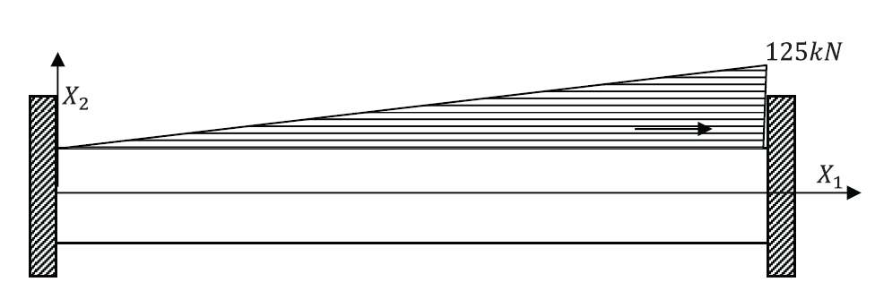
Example 5: Beam Under Axial Load with Displacement Boundary Conditions
A beam fixed at both ends is under a triangular axial load with a maximum value of 125 kN/m at  . The beam’s length, width, and height are 5, 0.25, and 0.5 m, respectively. Young’s modulus is 20 GPa. Ignore the effect of Poisson’s ratio. Find the displacement function of this beam along with the stress distribution along the length of the beam. Draw the contour plot of and the vector plot of the displacement along the beam.
SOLUTION
The displacement vector function of the beam has the form:
![\[u=\left(\begin{array}{c}u_1(X_1)\\0\\0\end{array}\right)\]](https://engcourses-uofa.ca/wp-content/ql-cache/quicklatex.com-c227e7217057c0d62a6edfef4ef9a61a_l3.png "Rendered by QuickLaTeX.com")
The only nonzero strain component is  :
:
![\[\varepsilon_{11}=\frac{\mathrm{d}u_1}{\mathrm{d}X_1}\]](https://engcourses-uofa.ca/wp-content/ql-cache/quicklatex.com-47875186beb4c4f06b5ddb7f9ae9ad91_l3.png "Rendered by QuickLaTeX.com")
Ignoring the effect of Poisson’s ratio, the only nonzero stress component is :
![\[\sigma_{11}=E\varepsilon_{11}=E\frac{\mathrm{d}u_1}{\mathrm{d}X_1}\]](https://engcourses-uofa.ca/wp-content/ql-cache/quicklatex.com-c7b544cfb80eb3237da11993baa0fc37_l3.png "Rendered by QuickLaTeX.com")
The distributed axial load follows the equation:
![\[p=125\frac{X_1}{L}\]](https://engcourses-uofa.ca/wp-content/ql-cache/quicklatex.com-6e30c7ac03a1e773e4e1fdcaca90acfd_l3.png "Rendered by QuickLaTeX.com")
The equilibrium equation (Equation 12) for beams under axial loading can be used with constant  to write:
![\[EA\frac{\mathrm{d}^2u_1}{\mathrm{d}X_1^2}=-125\frac{X_1}{L}\]](https://engcourses-uofa.ca/wp-content/ql-cache/quicklatex.com-5a5ba9135a9d52c51cf5f5878cd7b6fa_l3.png "Rendered by QuickLaTeX.com")
The boundary conditions are:
![\[\begin{split}@X_1=0 & :u_1=0\\@X_1=L & :u_1=0\end{split}\]](https://engcourses-uofa.ca/wp-content/ql-cache/quicklatex.com-ead367af3a8671113e8662ec348b6786_l3.png "Rendered by QuickLaTeX.com")
Therefore, the solution to the above ordinary differential equation yields the following forms for  , , and the normal force
  :
:
![\[u_1=\frac{125(X_1L^2-X_1^3)}{6EAL}\qquad \sigma_{11}=\frac{125(L^2-3X_1^2)}{6AL}\qquad N=\frac{125(L^2-3X_1^2)}{6L}\]](https://engcourses-uofa.ca/wp-content/ql-cache/quicklatex.com-cd4b918bf8430319baf7941e2e11d7c4_l3.png "Rendered by QuickLaTeX.com")
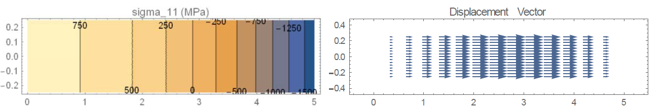
The required contour plots and the Mathematica code used are below.
View Mathematica Code
Clear[u,x,L,EA,Ee,A]
EA=Ee*A;
u1=u[x]/.x->0;
u2=u[x]/.x->L;
Normalf=EA*D[u[x]];
qnormal=125*x/L;
s=DSolve[{EA*u''[x]==-qnormal,u1==0,u2==0},u,x]
u=u[x]/.s[[1]]
s11=Ee*D[u,x]
Normalf=Normalf/.s[[1]];
Ee=20000;
A=0.25*0.5;
L=5;
disp={u,0}
ContourPlot[s11,{x,0,5},{X2,-0.25,0.25},AspectRatio->0.25,ContourLabels->True,PlotLabel->"sigma_11 (MPa)"]
VectorPlot[disp,{x,0,5},{X2,-0.25,0.25},AspectRatio->0.25,PlotLabel->"Displacement Vector"]
View Python Code
from sympy import *
from numpy import *
import sympy as sp
import numpy as np
import matplotlib.pyplot as plt
sp.init_printing(use_latex = "mathjax")
A, L, x , EA, E = symbols("A L x EA E")

def plotContour(f, limits, title):
    x1, xn, y1, yn = limits
    dx, dy = 10/100*(xn-x1),10/100*(yn - y1)
    xrange = np.arange(x1,xn+dx,dx)
    yrange = np.arange(y1,yn+dy,dy)
    X, Y = np.meshgrid(xrange, yrange)
    lx, ly = len(xrange), len(yrange)
    F = lambdify((x,X2),f)
    # if F is constant, then generates array
    # if F generates array, doesn't change anything
    Z = F(X,Y)*np.ones(lx*ly).reshape(lx, ly)
    fig = plt.figure(figsize = (8,2))
    ax = fig.add_subplot(111)
    cp = ax.contourf(X,Y,Z)
    fig.colorbar(cp)
    plt.title(title)

def plotVector(f, limits, title):
    fx, fy = [lambdify((x,X2),fi) for fi in f]
    x1, xn, y1, yn = limits
    dx, dy = 10/100*(xn-x1),10/100*(yn-y1)
    xrange = np.arange(x1,xn,dx)
    yrange = np.arange(y1,yn,dy)
    X, Y = np.meshgrid(xrange, yrange)
    dxplot, dyplot = fx(X,Y), fy(X,Y)
    fig = plt.figure(figsize = (7.5,2))
    ax = fig.add_subplot(111)
    ax.quiver(X, Y, dxplot, dyplot)
    plt.title(title)

u = Function("u")
EA = E * A
u1 = u(x).subs(x,0)
u2 = u(x).subs(x,L)
Normalf = EA * u(x).diff(x)
qnormal = 125 * x/L
display("Only non-zero stress component: ", Normalf)
display("Distributed axial Load: ", qnormal)
s = dsolve(EA * u(x).diff(x,2) + qnormal, u(x), ics = {u1:0, u2:0})
u = s.rhs
s11 = E * u.diff(x)
Normalf = EA * u.diff(x)
display("u_1, sigma_11 and Normal force: ", u, s11, Normalf)
s11 = s11.subs({E:20000, A:0.125, L:5})
u = u.subs({E:20000, A:0.125, L:5})
disp = Matrix([[u], [0]])
plotContour(s11, [0,5,-0.25,0.3], "sigma_11")
plotVector(disp, [0,5,-0.25,0.3], "Displacement Vector")
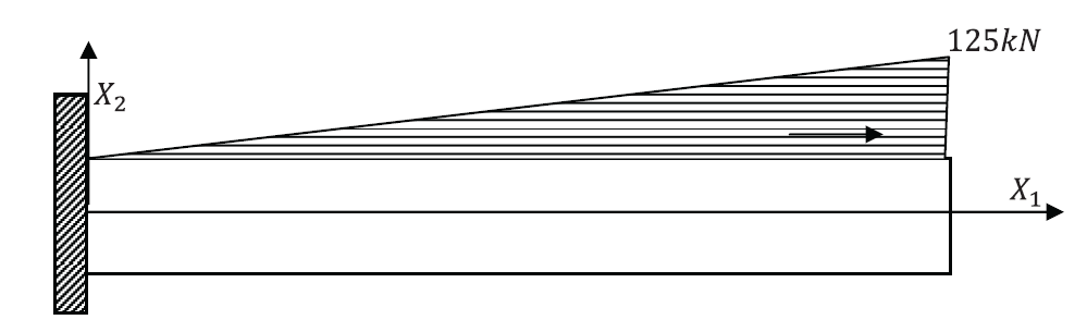
Example 6: Beam Under Axial Load with Displacement and Stress Boundary Conditions
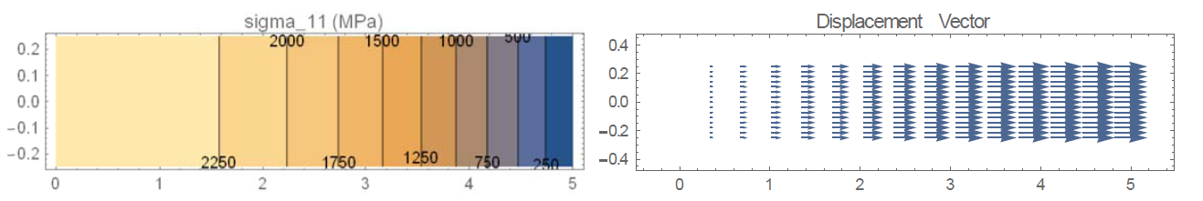
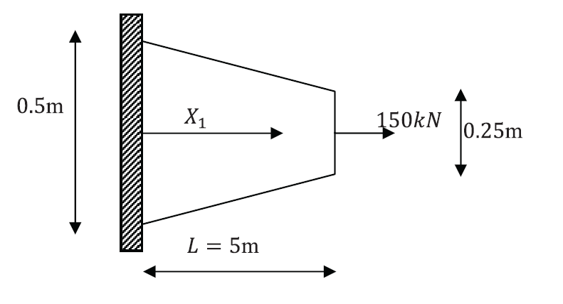
The shown beam has one fixed end and one free end. The beam is under a triangular axial load with a maximum value of 125kN/m at  . The beam’s length, width, and height are 5, 0.25, and 0.5m, respectively. Young’s modulus is 20 GPa. Ignore the effects of Poisson’s ratio and find the displacement function of this beam along with the stress distribution. Draw the contour plots of and the vector plot of the displacement.
axial 2
. The beam’s length, width, and height are 5, 0.25, and 0.5m, respectively. Young’s modulus is 20 GPa. Ignore the effects of Poisson’s ratio and find the displacement function of this beam along with the stress distribution. Draw the contour plots of and the vector plot of the displacement.
axial 2
SOLUTION:
The displacement vector function of the beam has the form:
The only nonzero strain component is :
Ignoring the effect of Poisson’s ratio, the only nonzero stress component is :
The distributed axial load follows the equation:
The equilibrium equation (Equation 12) for beams under axial loading can be used with constant to write:
The boundary conditions are:
![\[\begin{split}@X_1=0 & :u_1=0\\@X_1=L & :\sigma_{11}=E\frac{\mathrm{d}u_1}{\mathrm{d}X_1}=0\end{split}\]](https://engcourses-uofa.ca/wp-content/ql-cache/quicklatex.com-87d9f2740f03aec31e478265ede15f45_l3.png "Rendered by QuickLaTeX.com")
Therefore, the solution to the above ordinary differential equation yields the following forms for , , and the normal force :
![\[u_1=\frac{125(3X_1L^2-X_1^3)}{6EAL}\qquad \sigma_{11}=\frac{125(3L^2-3X_1^2)}{6AL}\qquad N=\frac{125(3L^2-3X_1^2)}{6L}\]](https://engcourses-uofa.ca/wp-content/ql-cache/quicklatex.com-f61518d0a5511d6b2425771f70e883f7_l3.png "Rendered by QuickLaTeX.com")
The required contour plots and the Mathematica code used are below. Compare the plots with the previous example.
The required contour plots and the Mathematica code used are below.
View Mathematica Code
Clear[u,x,L,EA,Ee,A]
EA=Ee*A;
u1=u[x]/.x->0;
BC2=D[u[x],x]/.x->L;
Normalf=EA*D[u[x]];
qnormal=125*x/L;
s=DSolve[{EA*u''[x]==-qnormal,u1==0,BC2==0},u,x]
u=u[x]/.s[[1]]
s11=Ee*D[u,x]
Normalf=Normalf/.s[[1]];
Ee=20000;
A=0.25*0.5;
L=5;
disp={u,0}
ContourPlot[s11,{x,0,5},{X2,-0.25,0.25},AspectRatio->0.25,ContourLabels->True,PlotLabel->"sigma_11 (MPa)"]
VectorPlot[disp,{x,0,5},{X2,-0.25,0.25},AspectRatio->0.25,PlotLabel->"Displacement Vector"]
View Python Code
from sympy import *
from numpy import *
import sympy as sp
import numpy as np
import matplotlib.pyplot as plt
sp.init_printing(use_latex = "mathjax")
A, L, x , EA, E = symbols("A L x EA E")

def plotContour(f, limits, title):
    x1, xn, y1, yn = limits
    dx, dy = 10/100*(xn-x1),10/100*(yn - y1)
    xrange = np.arange(x1,xn+dx,dx)
    yrange = np.arange(y1,yn+dy,dy)
    X, Y = np.meshgrid(xrange, yrange)
    lx, ly = len(xrange), len(yrange)
    F = lambdify((x,X2),f)
    # if F is constant, then generates array
    # if F generates array, doesn't change anything
    Z = F(X,Y)*np.ones(lx*ly).reshape(lx, ly)
    fig = plt.figure(figsize = (8,2))
    ax = fig.add_subplot(111)
    cp = ax.contourf(X,Y,Z)
    fig.colorbar(cp)
    plt.title(title)

def plotVector(f, limits, title):
    fx, fy = [lambdify((x,X2),fi) for fi in f]
    x1, xn, y1, yn = limits
    dx, dy = 10/100*(xn-x1),10/100*(yn-y1)
    xrange = np.arange(x1,xn,dx)
    yrange = np.arange(y1,yn,dy)
    X, Y = np.meshgrid(xrange, yrange)
    dxplot, dyplot = fx(X,Y), fy(X,Y)
    fig = plt.figure(figsize = (7.5,2))
    ax = fig.add_subplot(111)
    ax.quiver(X, Y, dxplot, dyplot)
    plt.title(title)

u = Function("u")
EA = E * A
u1 = u(x).subs(x,0)
BC2 = u(x).diff(x).subs(x,L)
Normalf = EA * u(x).diff(x)
qnormal = 125 * x/L
display("Only non-zero stress component: ", Normalf)
display("Distributed axial Load: ", qnormal)
s = dsolve(EA * u(x).diff(x,2) + qnormal, u(x), ics = {u1:0, BC2:0})
u = s.rhs
s11 = E * u.diff(x)
Normalf = EA * u.diff(x)
display("u_1, sigma_11 and Normal force: ", u, s11, Normalf)
s11 = s11.subs({E:20000, A:0.125, L:5})
u = u.subs({E:20000, A:0.125, L:5})
disp = Matrix([[u], [0]])
plotContour(s11, [0,5,-0.25,0.25], "sigma_11")
plotVector(disp, [0,5,-0.25,0.25], "Displacement Vector")
Example 7: Beam Under Axial Load With Varying Cross Sectional Area
The shown beam has a varying circular cross sectional area with a radius  units at the top varying linearly to
  unit at the bottom. The beam is used to carry a concentrated load
  and has a weight density \rho. Young’s modulus
  units. Find the vertical displacement field of the beam.
SOLUTION:
Since the beam has a varying cross sectional area, this induces a varying vertical load due to the beam’s own weight. The radius  and the area
  vary with according to the equations:
![\[r=2-\frac{X_1}{L}\qquad A=\pi\left(2-\frac{X_1}{L}\right)^2\]](https://engcourses-uofa.ca/wp-content/ql-cache/quicklatex.com-5c6964b66aa8e50831b40026a90afff2_l3.png "Rendered by QuickLaTeX.com")
Similar to the two previous examples, the only nonzero strain component is and ignoring Poisson’s ratio we get:
![\[\varepsilon_{11}=\frac{\mathrm{d}u_1}{\mathrm{d}X_1}\qquad \sigma_{11}=E\varepsilon_{11}=E\frac{\mathrm{d}u_1}{\mathrm{d}X_1}\]](https://engcourses-uofa.ca/wp-content/ql-cache/quicklatex.com-d858707bd166d706667ce012eafabd56_l3.png "Rendered by QuickLaTeX.com")
where is the unknown displacement component along the axis . The equilibrium equation (Equation 12) for beams under axial loading can be used with varying EA to write:
![\[E\frac{\mathrm{d}A}{\mathrm{d}X_1}\frac{\mathrm{d}u_1}{\mathrm{d}X_1}+EA\frac{\mathrm{d}^2u_1}{\mathrm{d}X_1^2}+\rho A=0\]](https://engcourses-uofa.ca/wp-content/ql-cache/quicklatex.com-d82cc2ef9729d13ac62811ed252ffb01_l3.png "Rendered by QuickLaTeX.com")
Substituting for in the above equation we get:
![\[E\frac{\pi}{2}\left(\frac{X_1}{4}-2\right)\frac{\mathrm{d}u_1}{\mathrm{d}X_1}+E\pi\left(2-\frac{X_1}{4}\right)^2\frac{\mathrm{d}^2u_1}{\mathrm{d}X_1^2}+\pi\rho\left(2-\frac{X_1}{4}\right)^2=0\]](https://engcourses-uofa.ca/wp-content/ql-cache/quicklatex.com-007e863523b43e6ae646199a6e626552_l3.png "Rendered by QuickLaTeX.com")
The boundary conditions are:
![\[\begin{split}@X_1=0 & :u_1=0\\@X_1=L & :\sigma_{11}=E\frac{\mathrm{d}u_1}{\mathrm{d}X_1}=\frac{P}{A}\bigg|_{X_1=L}\end{split}\]](https://engcourses-uofa.ca/wp-content/ql-cache/quicklatex.com-bb42cdbdf56ae25d58623cfa23cc8f62_l3.png "Rendered by QuickLaTeX.com")
Mathematica can be used to solve the above differential equation to find the solution for as follows:
![\[u_1=\frac{-12PX_1-112\pi\rho X_1+24 \pi\rho X_1^2-\pi\rho X_1^3}{6E\pi(X_1-8)}\]](https://engcourses-uofa.ca/wp-content/ql-cache/quicklatex.com-ddb287268520f328e1667e43033008d0_l3.png "Rendered by QuickLaTeX.com")
View Mathematica Code
Clear[L,A,Al,ro,Ee,u]
L=4;
A=Pi*(2-x/L)^2;
Al=A/.x->L;
s=DSolve[{D[Ee*A*u'[x],x]+ro*A==0,u[0]==0,u'[L]==P/Ee/Al},u,x]
View Python Code
from sympy import *
from numpy import *
import sympy as sp
import numpy as np
sp.init_printing(use_latex = "mathjax")
L, x , A, Al, ro, E, u, pi, P= symbols("L x A Al rho E u pi P")
u = Function("u")
u1 = u(x).subs(x,0)
u2 = u(x).diff(x).subs(x,L)
A = pi*(2-x/L)**2
display("Area: ", A)
Al = A.subs(x,L)
s = dsolve((E*A*u(x).diff(x)).diff(x) + ro * A, u(x), ics = {u1:0, u2:P/E/Al})
display(s.subs(L, 4))
You can now copy and paste the following code into Mathematica to see the effect of changing the density and the external load on the displacement function produced for  and
and  . What is the combination of
  and that would produce an almost linear displacement field?
View Mathematica Code
Clear[u,x,Ee,P,L,A]
Manipulate[Ee=1000;
L=4;
A=Pi*(2-x/L)^2;
Al=A/.x->L;
s=DSolve[{D[Ee*A*u'[x],x]+ro*A==0,u[0] ==0,u'[L] ==P/Ee/Al},u,x];
s=u/.s[[1]];
Plot[s[x],{x,0,L}],{P,0,500},{ro,0,100}]
View Python Code
%matplotlib notebook
from sympy import *
from numpy import *
import sympy as sp
import numpy as np
import matplotlib.pyplot as plt
from matplotlib.widgets import Slider
sp.init_printing(use_latex = "mathjax")
L, x , A, Al, ro, E, u, pi, P= symbols("L x A Al rho E u pi P")
u = Function("u")
u1 = u(x).subs(x,0)
u2 = u(x).diff(x).subs(x,L)
A = pi*(2-x/L)**2
Al = A.subs(x,L)
s = dsolve((E*A*u(x).diff(x)).diff(x) + ro * A, u(x), ics = {u1:0, u2:P/E/Al})
s = s.rhs
s = s.subs(L,4)
initial = s.subs({ro:100, P:500, E:1000, pi:np.pi})
fig = plt.figure()
ax = fig.add_subplot(111)
x1 = np.arange(0,4.1,1)
s_list = [initial.subs({x:i}) for i in x1]
#Initial PLot
ax.plot(x1, s_list)
def Update_func(event):
    new = s.subs({ro:slider1.val, P:slider2.val, E:1000, pi:np.pi})
    newx = np.arange(0,4.1,1)
    new_s_list = [new.subs({x:i}) for i in newx]
    ax.clear()
    ax.plot(newx, new_s_list)
plt.subplots_adjust(left = 0.1, bottom = 0.45)
roslider = plt.axes([0.2,0.2,0.5,0.03])
Pslider = plt.axes([0.2,0.15,0.5,0.03])
slider1 = Slider(roslider, 'ro', 0, 100, valinit = 100, valstep = 1)
slider2 = Slider(Pslider, 'P', 0, 500, valinit = 500, valstep = 1)
slider1.on_changed(Update_func)
slider2.on_changed(Update_func)

plt.show()
Problems
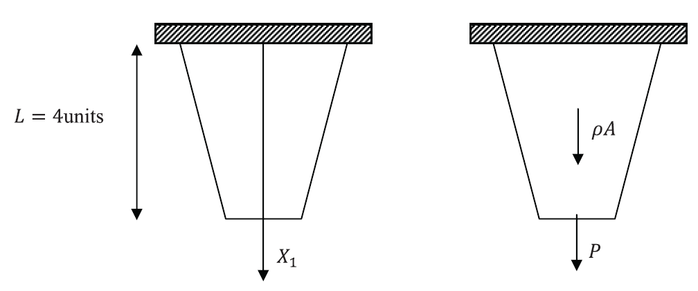
- Use Mathematica to solve the Euler Bernoulli beam and the Timoshenko beam equations (shear, moment, rotation (slope), and deflection) for the beams shown in the following figure (assume values for the loads and material constants). Also, find the maximum deflection associated with the loads shown.
- Rewrite the final equations presented for the Euler Bernoulli beam and the Timoshenko beam assuming that the cross-sectional area parameters I and A are not constant.
- Conduct a literature search to find the values of the shear coefficient k of the Timoshenko beam for different cross-sectional shapes. (Square, circle, I beam etc.)
- A beam is 6m long with a rectangular cross-sectional area whose width and height are 0.25m and 0.5m, respectively. Young’s modulus is 20GPa. Ignore the effect of Poisson’s ratio. A distributed load of a value 125kN/m is applied vertically downward. Compare the following between a simple beam and a fixed-ends beam:
- Deflection, bending moment, and shearing force distribution along the beam.
- , , , and the hydrostatic stress (Draw the contour plots and comment on the difference).
- The shown beam has a rectangular cross-sectional area with a width of 0.25m. The height of the beam varies linearly along its length as shown in the figure below. Young’s modulus is taken as 20GPa while the effect of Poisson’s ratio is ignored. Assume that the only nonzero component of the stress is and that plane sections perpendicular to the axis remain plane and perpendicular to the axis after deformation. Find the following:
- A generic form for the position and the displacement functions.
- The expression for the infinitesimal strain tensor components.
- The differential equation of equilibrium and its boundary conditions.
- Solve the differential equation of equilibrium to find the displacement of the beam at every point.
- Draw the contour plots of .
- Draw the vector plot of the displacement vector
 .
.
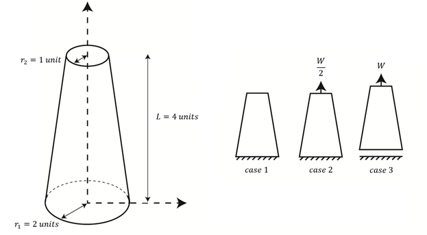
- The shown beam structure has a circular cross sectional area with radius of 2m at the bottom varying linearly to 1m at the top. The length of the structure is 4m. A crane is used to carry it from the top. Consider the weight density of the member as 10 N/m^3 and Young’s modulus of 1000 N/m^2. Ignore Poisson’s ratio and assume that the only nonzero component of the stress is the normal stress in the vertical direction and that it is uniformly distributed in the cross section. Find the displacement function of the beam, the total elongation or contraction, and the distribution of the nonzero normal stress component in the following cases:
- When the beam is resting on the ground.
- When the crane is carrying half the weight of the beam but the bottom of the beam is still on the ground.
- When the beam is suspended in the air.
- A cantilever beam with a rectangular cross section is subjected to a uniformly distributed load. The length of the beam is 5 m, its width and height are respectively 400 mm and 500 mm and the distributed load is equal to 15 KN/m. A rigid block is located under the free end of the beam and a gap equal to 10 mm exists between the free end and the rigid block. Consider the Young’s modulus as 20 GPa and find the following:
- the reaction force of the rigid block.
- the deflection of the neutral axis of the beam.
- the displacement field inside the beam.
- the stress component inside the beam. Draw the contour plots of .
This is educational ressources of highest quality. Good job.