Engineering at Alberta Courses » Description of Motion and Simple Examples

Displacement and Strain: Description of Motion and Simple Examples

Learning Outcomes

Define the mathematical description of motion as a mathematical function that relates the material points of an object in an “undeformed” or “pre-deformed” state to its “deformed” state.
Identify the following examples of deformation functions: Rigid body displacement, rigid body rotation, rigid body motion, Uniform extension and contraction, Simple shear, pure shear.

Description of Motion

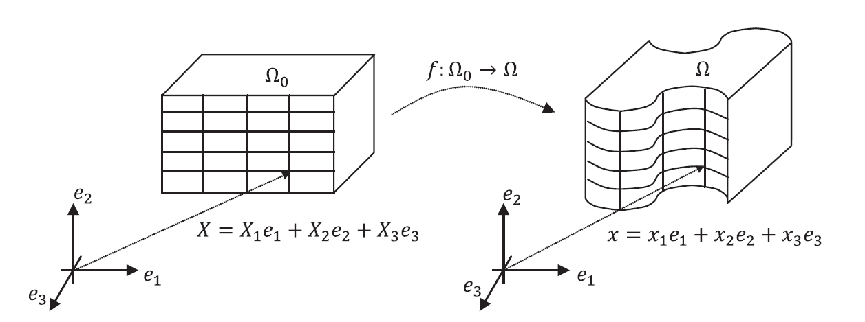
The geometry of a continuum body can be represented mathematically by “embedding” it in a Euclidean Vector Space $\mathbb{R}^3$ where every material point in the body can be represented by a unique vector in the space. We denote the set of vectors corresponding to the material points by $\Omega\subset\mathbb{R}^3$ . The embedding is called a “configuration”. An analyst is usually interested in comparing a “deformed” configuration $\Omega\subset\mathbb{R}^3$ with an “undeformed” or a “reference” configuration $\Omega_0\subset\mathbb{R}^3$ . Traditionally, elements of the deformed configuration are denoted by $x\in\Omega$ while elements in the reference configuration are denoted by $X\in\Omega_0$ . The deformed configuration can be assumed to be a function $f:X\in\Omega_0\rightarrow x\in\Omega$ such that $x=f(X)$ (Figure 1). In the majority of continuum mechanics applications, the following are the major restrictions on the possible choices of the position function $f$ .

First, we assume that the deformation between configurations preserves the distinction between material points, i.e., that material is not flattened out or lost during configuration. This restricts $f$ to be bijective.
Second, we assume that material points don’t change their neighbours, i.e., no cracks or rearrangement of material points occur during deformation. This restricts $f$ to be continuous.
In most applications we add the third restriction of being “smooth” or “differentiable” on the possible choices for $f$ . This ensures that straight lines on the reference configuration deform into smooth curves in the deformed configuration. This allows the calculation of derivatives and the definition of “strain”.

The displacement function of the body (termed the displacement field) is denoted by the function $u:\Omega_0\rightarrow \mathbb{R}^3$ such that:

$\emph{u(X) = x - X = f(x) - X}$

A geometric object is embedded in $\mathbb{R}^3: \Omega_0$ is the set of vectors representing the reference configuration, while $\Omega$ is the set representing the deformed configuration.

In the following section a few simple examples of deformations along with their position and displacement functions are presented.

Rigid Body Displacement

A rigid body displacement is represented by a constant displacement vector at every point. The new (deformed) position $x\in\mathbb{R}^3$ of every point is related to the old (reference) position $X\in\mathbb{R}^3$ as follows:

$\emph{ x = X + c}$

where

$\emph{c} \hspace{2mm} \in \hspace{2mm} \mathbb{R}^3$

is a constant vector. The displacement field at every point is the difference between the deformed and reference positions and is constant:

$\emph{ u = x - X = c}$

Change the components of the vector $\emph{c}$ in the following tool to view its effect on the displacement of the cuboid.

Rigid Body Rotation

A rigid body rotation is represented by a rotation matrix $Q\in\mathbb{M}^3$ ( see Orthogonal Tensors ) such that the new (deformed) position $x\in\mathbb{R}^3$ of every point is equal to the rotation matrix Q multiplied by the old (reference) position $X\in\mathbb{R}^3$ as follows:

$\emph{x = QX}$

The displacement field at every point is the difference between the deformed and reference positions:

$\emph{u = x - X = QX - X = (Q-I)X}$

Recall that any rotation matrix can be viewed as consecutive rotations around each of the basis vectors of the coordinate system. Clockwise rotations with angles $\theta_a, \theta_b, \theta_c$ around the basis vectors $e_1$ , $e_2$ and $e_3$ are given by the following matrices $Q_a$ , $Q_b$ and $Q_c$ , respectively:

$Q_a = \begin{pmatrix} 1 & 0 & 0 \\ 0 & \cos(\theta_a) & \sin(\theta_a) \\ 0 & -\sin(\theta_a) & cos(\theta_a) \\ \end{pmatrix}$

$Q_b = \begin{pmatrix} \cos(\theta_b) & 0 & -\sin(\theta_b) \\ 0 & 1 & 0 \\ \sin(\theta_b) & 0 & cos(\theta_b) \\ \end{pmatrix}$

$Q_c = \begin{pmatrix} \cos(\theta_c) & \sin(\theta_c) & 0 \\ -\sin(\theta_c) & \cos(\theta_c) & 0 \\ 0 & 0 & 1 \\ \end{pmatrix}$

It is important to notice that the order of rotation changes the final position of the rotated object. The rotation matrix $Q_1 = Q_c Q_b Q_a$ describes a rotation of $\theta_a$ around $e_1$ followed by a rotation of $\theta_b$ around $e_2$ and finally a rotation of $\theta_c$ around $e_3$ . On the other hand, the rotation matrix $Q_2 = Q_c Q_b Q_a$ describes a rotation of $\theta_c$ around $e_3$ followed by a rotation of $\theta_b$ around $e_2$ and finally a rotation of $\theta_a$ around $e_1$ . In general: $Q_1 \neq Q_2$ . In the following example, the red box represents the original box after rotation around the basis vectors. Try it out: rotate the box 90 degrees around $\emph{x}$ and then slowly rotate it around $\emph{y}$ . This order is applied to the image on the left. The order of rotation applied to the one on the right is reversed! Compare the two orders of rotation. The overall matrix of transformation is displayed at the bottom of each image.

Rigid Body Motion

A rigid body motion is a combination of both a rigid body displacement and a rigid body rotation such that the deformed position $x\in\mathbb{R}^3$ is function of the reference position $X\in\mathbb{R}^3$ as follows:

$\emph{x = QX + c}$

where $\emph{Q} \hspace{2mm} \in \hspace{2mm} \mathbb{R}^3$ is a rotation matrix and $\emph{c} \hspace{2mm} \in \hspace{2mm} \mathbb{R}^3$ is a vector representing the rigid body displacement. The displacement field can be expressed as:

$\emph{u = x - X = (Q-I)X + c}$

In component form, the relationship between the vectors $\emph{x}$ and $\emph{X}$

can be written as follows:

$\begin{pmatrix} x_1 \\ x_2 \\ x_3 \\ \end{pmatrix} = \begin{pmatrix} Q_{11} & Q_{12} & Q_{13} \\ Q_{21} & Q_{22} & Q_{23} \\ Q_{31} & Q_{32} & Q_{33} \\ \end{pmatrix} \begin{pmatrix} X_1 \\ X_2 \\ X_3 \\ \end{pmatrix} + \begin{pmatrix} c_1 \\ c_2 \\ c_3 \\ \end{pmatrix}$

Note that in some numerical analysis software and tools, the above relationship adopts the following form:

$\begin{pmatrix} x_1 \\ x_2 \\ x_3 \\ 1 \\ \end{pmatrix} = \begin{pmatrix} Q_{11} & Q_{12} & Q_{13} & c_1 \\ Q_{21} & Q_{22} & Q_{23} & c_2 \\ Q_{31} & Q_{32} & Q_{33} & c_3 \\ 0 & 0 & 0 & 1 \\ \end{pmatrix} \begin{pmatrix} X_1 \\ X_2 \\ X_3 \\ 1 \\ \end{pmatrix}$

Change the angles of rotation and the components of the vector $c$ in the following tool to see the effect on the final position of the cube.

Uniform Extension and Contraction

A uniform extension or contraction can be characterized by three positive parameters $k_1$ , $k_2$ , and $k_3\in\mathbb{R}^3$ that represent the ratios between the three vector components in the deformed configuration to the components in the reference configuration:

$\begin{pmatrix} x_1 \\ x_2 \\ x_3 \\ \end{pmatrix} = \begin{pmatrix} k_1 & 0 & 0 \\ 0 & k_2 & 0 \\ 0 & 0 & k_3 \\ \end{pmatrix} \begin{pmatrix} X_1 \\ X_2 \\ X_3 \\ \end{pmatrix} = \begin{pmatrix} k_1 X_1 \\ k_2 X_2 \\ k_3 X_3 \\ \end{pmatrix}$

Note that the relationship can be written as a linear transformation $\emph{x = MX}$ where $\emph{M} \hspace{2mm} \in \hspace{2mm} \mathbb{M}^3$ has the form:

$M = \begin{pmatrix} k_1 & 0 & 0 \\ 0 & k_2 & 0 \\ 0 & 0 & k_3 \\ \end{pmatrix}$

In the following example, you can vary the values of $k_1$ , $k_2$ ,and $k_3$ to see the effect on the deformation of a cube. What values constitute compression and what values constitute tension? Also, what does it mean that the value of $k_i$ is equal to 1 or 0?

Simple Shear

The simple shear motion is described by a shearing angle along a certain direction and perpendicular to another direction. The following relationship describes a simple shear motion in which the planes parallel to the basis vectors $e_2$ and $e_3$ are sheared in the direction of $e_1$ :

$\begin{pmatrix} x_1 \\ x_2 \\ x_3 \\ \end{pmatrix} = \begin{pmatrix} 1 & \tan(\theta) & 0 \\ 0 & 1 & 0 \\ 0 & 0 & 1 \\ \end{pmatrix} \begin{pmatrix} X_1 \\ X_2 \\ X_3 \\ \end{pmatrix} = \begin{pmatrix} X_1 + \tan(\theta)X_2 \\ X_2 \\ X_3 \\ \end{pmatrix}$

Note that the relationship can be written as a linear transformation $\emph{ x = MX}$ where $\emph{M} \hspace{2mm} \in \hspace{2mm} \mathbb{M}^3$ Note that the relationship can be written as a linear transformation has the form:

$M = \begin{pmatrix} 1 & \tan(\theta) & 0 \\ 0 & 1 & 0 \\ 0 & 0 & 1 \\ \end{pmatrix}$

In the following example, change the values of $\theta_{xy}$ , $\theta_{yz}$ and $\theta_{xz}$ in the matrix $M$ :

$M = \begin{pmatrix} 1 & \tan(\theta_{xy}) & \tan(\theta_{xz}) \\ 0 & 1 & \tan(\theta_{yz}) \\ 0 & 0 & 1 \\ \end{pmatrix}$

and observe the effect on the deformation $\emph{x = MX}$ . The term simple shear applies to the deformations when only one of the angles $\theta_{xy}$ , $\theta_{yz}$ , and $\theta_{xz}$ is non-zero.

Pure Shear

The following relationship describes a pure shear motion with an angle $\theta$ in the plane of $e_1$ and $e_2$ :

$\begin{pmatrix} x_1 \\ x_2 \\ x_3 \\ \end{pmatrix} = \begin{pmatrix} 1 & \tan(\theta/2) & 0 \\ \tan(\theta/2) & 1 & 0 \\ 0 & 0 & 1 \\ \end{pmatrix} \begin{pmatrix} X_1 \\ X_2 \\ X_3 \\ \end{pmatrix} = \begin{pmatrix} X_1 + \tan(\theta/2)X_2 \\ \tan(\theta/2)X_1 + X_2 \\ X_3 \\ \end{pmatrix}$

Note that the relationship can be written as a linear transformation $\emph{x = MX}$ where $\emph{M} \hspace{2mm} \in \hspace{2mm} \mathbb{M}^3$ has the form:

$M = \begin{pmatrix} 1 & \tan(\theta/2) & 0 \\ \tan(\theta/2) & 1 & 0 \\ 0 & 0 & 1 \\ \end{pmatrix}$

The difference between pure shear and simple shear can be viewed in the following two dimensional example. Change the value of $\theta_{xy}$ to see the deformation of a rectangle under pure shear (on the left) and under simple shear (on the right). The matrix $M$ in each case is given underneath the figure:

In the following example, change the values of $\theta_{xy}$ , $\theta_{yz}$ , and $\theta_{xz}$ in the matrix $M$ :

$M = \begin{pmatrix} 1 & \tan(\theta_{xy/2}) & \tan(\theta_{xz/2}) \\ \tan(\theta_{xy/2}) & 1 & \tan(\theta{yz/2}) \\ \tan(\theta_{xz/2}) & t\tan(\theta_{yz/2}) & 1 \\ \end{pmatrix}$

and observe the effect on the deformation $\emph{x = MX}$ . The term pure shear applies to the deformations when only one of the angles $\theta_{xy}$ , $\theta_{yz}$ ,and $\theta_{xz}$ is non-zero.