
Finite Element Analysis: Examples and Problems
Comparison of Different Elements Under Bending
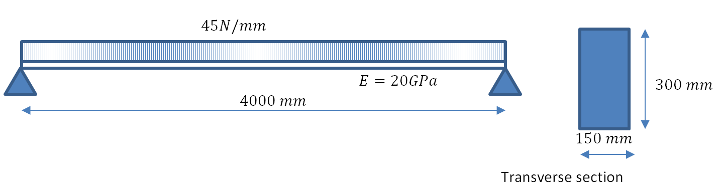
To compare the different elements described earlier, the simply supported beam with the distributed load shown in Figure 1 was modelled in the finite element analysis software ABAQUS with various different element types. The beam is supporting a distributed load  and has a Young’s modulus
  and a length
  . The beam was modelled as a 2D plane shell and meshed using 2D plane stress solid elements. Plane stress assumes that the thickness of the beam is small, allowing the material to freely deform in the third direction, thereby resulting in a zero stress components in the third direction
  . The third direction is the 150mm dimension in this case. The thickness of the plane stress element was set to 150mm, while the value of the pressure load applied was set to
  . The imposed boundary conditions are
  at one end and a roller support
  at the other end. Since this is a plane problem, specifying
  is redundant. The beam was modelled with various types of elements and mesh sizes. The maximum normal stress components
  at the top and bottom fibers of the beam at mid-span and the maximum vertical displacement
  were determined in response to the applied distributed load.
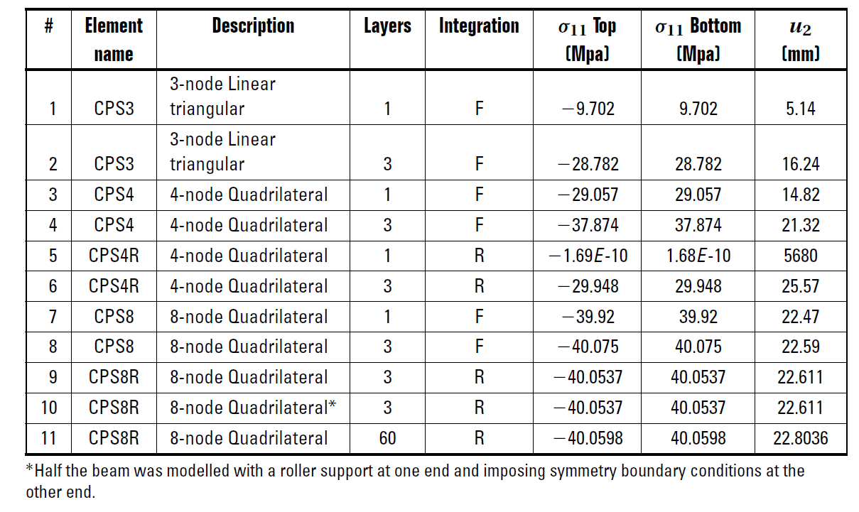
The following table compares the results for different elements with different mesh sizes measured by the number of elements (layers) in the direction of the second basis vector. Model 11 is a very fine mesh version of model 9 to show the effects of mesh refinement.
The results according to the Euler Bernoulli beam theory are as follows. Since no load is applied in the horizontal direction, the reaction in direction is equal to zero. The vertical reaction  at each end can be calculated as follows:
![\[R = \frac{wL}{2} = \frac{45 \times 4000}{2} = 90kN\]](https://engcourses-uofa.ca/wp-content/ql-cache/quicklatex.com-dfbf43d58e1145c25cb50777c9ef993d_l3.png "Rendered by QuickLaTeX.com")
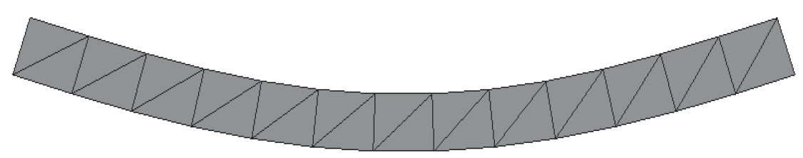
The reaction forces in all models matched the one calculated above. The deformed shape (Figure 2) in all the models matches the shape that is expected based on the loading and boundary conditions.
The maximum displacement (obtained in the mid-span) using the Euler Bernoulli beam theory for simply supported beam with a distributed load are given by:
![\[u_{max} = \frac{5wL^4}{384EI} = \frac{5 \times 45 \times (4000)^4}{384 \times 20000 \times 3.375 \times 10^8} = 22.2 mm\]](https://engcourses-uofa.ca/wp-content/ql-cache/quicklatex.com-e77ba1e852a2bc05e11c1f6744d14d82_l3.png "Rendered by QuickLaTeX.com")
where  is the moment of inertia for the rectangular cross section give by:
![\[I = \frac{150(300)^3}{12} = 3.375 \times 10^8 mm^4\]](https://engcourses-uofa.ca/wp-content/ql-cache/quicklatex.com-097952d021652535cf907d22a8aa99b5_l3.png "Rendered by QuickLaTeX.com")
The maximum bending moment for a simply supported beam is located at mid-span and is given by the following equation:
![\[M = \frac{wL^2}{8} = \frac{45(4000)^4}{8} = 9 \times 10^7 N \cdot mm\]](https://engcourses-uofa.ca/wp-content/ql-cache/quicklatex.com-42e48132298d87c4327007c286b8c749_l3.png "Rendered by QuickLaTeX.com")
The normal stress component at the bottom fibre corresponding to the maximum bending moment can be obtained as:
![\[\sigma_{11} = \frac{M \frac{t}{2}}{I} = \frac{9 \times 10^7 \times 150}{3.375 \times 10^8} = 40 MPa\]](https://engcourses-uofa.ca/wp-content/ql-cache/quicklatex.com-bd478076257d9563e1c012aa519ebe66_l3.png "Rendered by QuickLaTeX.com")
The Euler Bernoulli beam model predicts a linear stress profile with  at the top fibres. Notice that these results are not necessarily very accurate since the Euler Bernoulli beam theory assumes that plane sections prependicular to the neutral axis before deformation remain plane and perpendicular to the neutral axis after deformation.
Behaviour of Linear Triangular Elements
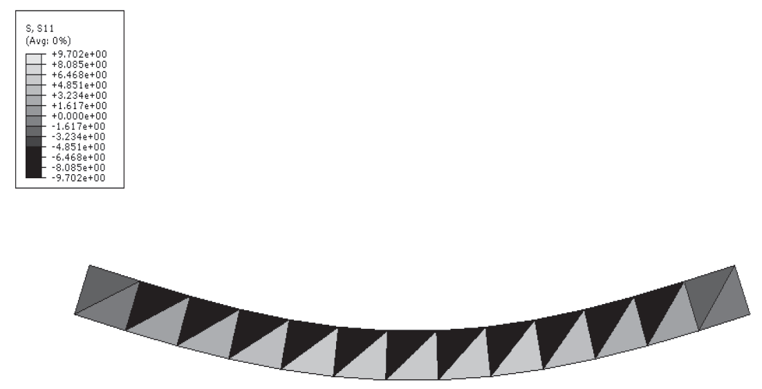
The linear triangular elements dramatically underestimate the stress and the displacement. These are constant strain elements, which is evident when viewing the stress contour plot without averaging across the elements (Figure 3). Linear triangular elements are not appropriate for bending (particularly when only one layer is used) because the strain in bending is not constant, but varies linearly from the top edge to the bottom edge. It is evident from the displacement that these elements produce a very stiff structure when only one layer is used. The result is improved when three layers of elements are used because the strain is forced to be constant over a smaller area, as opposed to constant across the entire cross section of the structure. Using these elements with a very fine mesh (60 layers) comes closer to the beam theory solution with  and
and  .
.
Behaviour of 4-Node Quadrilateral Elements
4-node quadrilateral elements offer an improved solution over the linear triangular elements; however, they are still relatively stiff due to shear locking (parasitic shear) described when the element was presented here. These elements allow the stress to vary linearly within the element. In that case, they allow a negative stress at the top and a positive stress at the bottom (Figure 4). Mesh refinement to three layers greatly improves the solution, producing results that approach the Euler Bernoulli beam solution.
 produced with a course mesh of linear quadrilateral elements.
Effect of Using Reduction Integration
Using one layer of the 4-node quadrilateral elements with reduced integration produces an extremely soft structure with wildly inaccurate results. The 4-node quadrilateral elements have
4 integration points. Using reduced integration, the number of integration points is reduced to one. This is not enough to capture the actual behaviour of the element and results in a very soft structure. The integration point is at the center of the element, which is at the neutral axis of the beam when one layer of elements is used. The stresses and strains in the models with a roller support at the right end (engineering beam theory) have zero stress at the neutral axis. So, the results suggest that the elements have zero (or close to zero) stress everywhere and an extremely high displacement. It is clear that a coarse mesh of the 4-node quadrilateral elements with reduced integration cannot be used to model a beam under bending. Refining the mesh to three layers produces much more reasonable results; however, the displacement is still overestimated, meaning that the modelled structure is still softer than the exact solution.
Behaviour of 8-Node Quadrilateral Elements
8-node quadrilateral elements produce very good results, even with only one layer of elements. The higher number of nodes and integration points allows these elements to model the stress distribution within the beam with only one element in the cross section. Mesh refinement to three layers produces a slightly softer structure, with results very close to the Euler-Bernoulli beam solution. Using reduced integration with the 8-node quadrilateral elements reduces the number of integration points from 9 to 4 with very little change in the results. Since there is very little change in the results, it would be advantageous to use reduced integration with these elements because the computational time is dramatically reduced. It is evident from the displacement results that the reduced integration 8-node quadrilateral elements have essentially reached a converged solution with a three-layer mesh. When compared to a 60-layer mesh (a huge increase in number of elements), very little change occurs in the results. It can also be noted that the change in the stress is much smaller than the change in the displacement between the two mesh sizes.
Symmetry and Concentrated Loads
In the cases where half the beam was modelled with a symmetry boundary condition imposed on the symmetry plane, the results are exactly the same as in the case with the same mesh and the full beam. This result is to be expected because the beam and the solution are symmetrical. The symmetry boundary condition that was imposed was to constrain the horizontal displacement along the entire symmetry plane  .
.
For the linear elastic material assumption, the equations of elasticity predict infinite values of the stress at the points where concentrated loads are applied. This indicates that the stress at such locations will never achieve convergence as the stress is unbounded. The boundary conditions used in this example impose a concentrated load at the corners of the beam, causing stress concentrations and a discontinuity in the deformation. The stresses further away from the concentrated load have converged, but since at the tip of the concentrated load, the predicted stresses from the elastic solution are infinite, then the finer the mesh used, the higher the values of the stress at this location. As shown in Figure 5, the stresses in the element where the concentrated reaction is applied are over 200 MPa, which is five times the maximum at the mid-span of the beam.
Conclusions
Analyzing this simple beam problem highlights the importance of choosing appropriate elements, integration procedures, and mesh sizes. It was seen that linear-triangular elements are not appropriate in bending unless an extremely fine mesh is used. This is because of their constant strain/stress condition. 4-node quadrilateral elements were seen to behave better than the triangular elements, but are still too stiff for this application when a coarse mesh is used. It was determined that the 8-node quadrilateral elements produce very good results for this application, even when a coarse mesh is used. The different behaviour of these elements is a result of their different shape functions. The analysis emphasizes the importance of understanding the shape functions used with each element and understanding how the elements will behave in a given situation. While reduced integration can save on computational time, it must be applied carefully. With the 4-node quadrilateral elements, reduced integration produced a very soft structure because the one integration point is not enough to capture the behaviour of a coarse mesh. It is evident that reduced integration should only be used with these elements if a finer mesh is used. The 8-node quadrilateral elements with reduced integration seem to be the best option for this application. Using a three-layer mesh, the results are very accurate. Using reduced integration and taking advantage of symmetry saves computational time without compromising the results. In the present example, with the relatively small number of elements, the computational time is not a big factor; however, it would be more important in a larger, more complex model necessitating a finer mesh. In that case, it would be beneficial to use reduced integration and to take advantage of symmetry wherever possible.
Examples and Problems
Example 1
Find the stiffness matrix and the nodal loads due to a traction vector and a body forces vector in a plane stress element of a linear elastic small deformations material whose Young’s modulus = 1 unit and Poisson’s ratio = 0.3. Use isoparametric formulation with exact integration, full integration, and finally, with reduced integration. The geometry and loading are shown below. The thickness of the element is assumed to be equal to 1 unit.
Solution
The mapping functions between the spatial coordinate system  and the element coordinate system
  are given by:
![\[x = \sum_{i=1}^4 N_ix_i = \frac{7 + \eta + 6\xi}{4}\]](https://engcourses-uofa.ca/wp-content/ql-cache/quicklatex.com-b294ffc6989a7eb94509bb0cfec340a6_l3.png "Rendered by QuickLaTeX.com")
![\[y = \sum_{i=1}^4 N_iy_i = \frac{18 + \eta(13-2\xi) + 3\xi}{10}\]](https://engcourses-uofa.ca/wp-content/ql-cache/quicklatex.com-c8a2c12310536aaf0ca65646bbc2fbad_l3.png "Rendered by QuickLaTeX.com")
The gradient of the mapping is given by:
![\[J = \begin{pmatrix} \frac{\partial x}{\partial \xi} & \frac{\partial x}{\partial \eta} \\ \frac{\partial y}{\partial \xi} & \frac{\partial y}{\partial \eta} \\ \end{pmatrix} = \begin{pmatrix} \frac{3}{2} & \frac{1}{4} \\ \frac{3-2\eta}{10} & \frac{13-2\eta}{10} \\ \end{pmatrix}\]](https://engcourses-uofa.ca/wp-content/ql-cache/quicklatex.com-2ff06c2e2618a47896e2f211b55958af_l3.png "Rendered by QuickLaTeX.com")
![\[J^{-1} = \begin{pmatrix} \frac{\partial \xi}{\partial x} & \frac{\partial \xi}{\partial y} \\ \frac{\partial \eta}{\partial x} & \frac{\partial \eta}{\partial y} \\ \end{pmatrix} = \frac{1}{75 + 2\eta - 12\xi} \begin{pmatrix} 52-8\xi & -10 \\ 4(-3+2\eta) & 60 \\ \end{pmatrix}\]](https://engcourses-uofa.ca/wp-content/ql-cache/quicklatex.com-dbb7eeebcd47b43ca1eb92701dc21962_l3.png "Rendered by QuickLaTeX.com")
The  matrix is given by:
![\[B = \begin{pmatrix} 1 & 0 & 0 & 0 \\ 0 & 0 & 0 & 1 \\ 0 & 1 & 1 & 0 \\ \end{pmatrix} \begin{pmatrix} \frac{\partial \xi}{\partial x} & \frac{\partial \eta}{\partial x} & 0 & 0 \\ \frac{\partial \xi}{\partial y} & \frac{\partial \eta}{\partial y} & 0 & 0 \\ 0 & 0 & \frac{\partial \xi}{\partial x} & \frac{\partial \eta}{\partial x} \\ 0 & 0 & \frac{\partial \xi}{\partial y} & \frac{\partial \eta}{\partial y} \\ \end{pmatrix} \begin{pmatrix} \frac{\partial N_1}{\partial \xi} & 0 & \frac{\partial N_2}{\partial \xi} & 0 & \frac{\partial N_3}{\partial \xi} & 0 \\ \frac{\partial N_1}{\partial \eta} & 0 & \frac{\partial N_2}{\partial \eta} & 0 & \frac{\partial N_3}{\partial \eta} & 0 \\ 0 & \frac{\partial N_1}{\partial \xi} & 0 & \frac{\partial N_2}{\partial \xi} & 0 & \frac{\partial N_3}{\partial \xi} \\ 0 & \frac{\partial N_1}{\partial \eta} & 0 & \frac{\partial N_2}{\partial \eta} & 0 & \frac{\partial N_3}{\partial \eta} \\ \end{pmatrix}\]](https://engcourses-uofa.ca/wp-content/ql-cache/quicklatex.com-8ad60a831e669b8a01fea7b3b61e323f_l3.png "Rendered by QuickLaTeX.com")
The stiffness matrix is given by:
![\[K = t \int_{-1}^1 \int_{-1}^1 B^T CB \det J d\xi d\eta\]](https://engcourses-uofa.ca/wp-content/ql-cache/quicklatex.com-c67606a80b603f6df837fc3120ecbb3a_l3.png "Rendered by QuickLaTeX.com")
Where  is the linear elastic isotropic plane stress constitutive relationship matrix. Exact integration produces the following stiffness matrix (units of force/length):
![\[K = \begin{pmatrix} 0.3228 & 0.1002 & -0.254 & 0.0002 & -0.1009 & -0.1437 & 0.032 & 0.0433 \\ 0.1002 & 0.3896 & 0.0277 & 0.0887 & -0.1437 & -0.1372 & 0.0159 & -0.3411 \\ -0.254 & 0.0277 & 0.7125 & -0.302 & -0.05 & 0.0319 & -0.4085 & 0.2424 \\ 0.0002 & 0.0887 & -0.302 & 0.785 & 0.0594 & -0.4343 & 0.2424 & -0.4395 \\ -0.1009 & -0.1437 & -0.05 & 0.0594 & 0.3911 & 0.0868 & -0.2403 & -0.0025 \\ -0.1437 & -0.1372 & 0.0319 & -0.4343 & 0.0868 & 0.4672 & 0.025 & 0.1043 \\ 0.032 & 0.0159 & -0.04085 & 0.2424 & -0.2403 & 0.025 & 0.6169 & -0.2833 \\ 0.0433 & -0.3411 & 0.2424 & -0.4395 & -0.0025 & 0.1043 & -0.2833 & 0.6763 \\ \end{pmatrix}\]](https://engcourses-uofa.ca/wp-content/ql-cache/quicklatex.com-6cf0a005151d248be02779134e3d0244_l3.png "Rendered by QuickLaTeX.com")
Setting  , full integration produces the following stiffness matrix (units of force/length):
![\[K = (K_1)_{\xi = \frac{-1}{\sqrt{3}}, \eta = \frac{-1}{\sqrt{3}}} + (K_1)_{\xi = \frac{1}{\sqrt{3}},\eta = \frac{-1}{\sqrt{3}}} + (K_1)_{\xi = \frac{-1}{\sqrt{3}}, \eta = \frac{1}{\sqrt{3}}} + (K_1)_{\xi = \frac{1}{\sqrt{3}}, \eta = \frac{1}{\sqrt{3}}}\]](https://engcourses-uofa.ca/wp-content/ql-cache/quicklatex.com-b32484a6aae8e83249e06b751ae605eb_l3.png "Rendered by QuickLaTeX.com")
![\[= \begin{pmatrix} 0.3226 & 0.1003 & -0.2536 & 0.0001 & -0.10129 & -0.1436 & 0.0322 & 0.0433 \\ 0.1003 & 0.389 & 0.0275 & 0.0896 & -0.1436 & -0.138 & 0.0158 & -0.3405 \\ -0.2536 & 0.0275 & 0.712 & -0.3019 & -0.0495 & 0.0318 & -0.4089 & 0.2425 \\ 0.0001 & 0.0896 & -0.3019 & 0.7839 & 0.0593 & -0.4332 & 0.2425 & -0.4403 \\ -0.1012 & -0.1436 & -0.0495 & 0.0593 & 0.3907 & 0.0869 & -0.24 & -0.0026 \\ -0.1436 & -0.138 & 0.0318 & -0.4332 & 0.0869 & 0.4662 & 0.0249 & 0.105 \\ 0.0322 & 0.0158 & -0.04089 & 0.2425 & -0.24 & 0.0249 & 0.6166 & -0.2832 \\ 0.0433 & -0.3405 & 0.2425 & -0.4403 & -0.0026 & 0.105 & -0.2832 & 0.6758 \\ \end{pmatrix}\]](https://engcourses-uofa.ca/wp-content/ql-cache/quicklatex.com-e861ae0cd0e366e3e7fc6206042ee2f5_l3.png "Rendered by QuickLaTeX.com")
Reduced integration produces the following stiffness matrix (units of force/length):
![\[K = 2 \times 2 \times (K_1)_{\xi=0,\eta = 0}\]](https://engcourses-uofa.ca/wp-content/ql-cache/quicklatex.com-3e676b6769e3e9e2f18a639f3b444af8_l3.png "Rendered by QuickLaTeX.com")
![\[= \begin{pmatrix} 0.2266 & 0.119 & -0.1223 & -0.0256 & -0.2266 & -0.119 & 0.1223 & 0.0256 \\ 0.119 & 0.2802 & 0.0018 & 0.2385 & -0.119 & -0.2802 & -0.0018 & -0.2385 \\ -0.1223 & 0.0018 & 0.5321 & -0.2667 & 0.1223 & -0.0018 & -0.5321 & 0.2667 \\ -0.0256 & 0.2385 & -0.2667 & 0.58 & 0.0256 & -0.2385 & 0.2667 & -0.58 \\ -0.2266 & -0.119 & 0.1223 & 0.0256 & 0.2266 & 0.119 & -0.1223 & -0.0256 \\ -0.119 & -0.2802 & -0.0018 & -0.2385 & 0.119 & 0.2802 & 0.0018 & 0.2385 \\ 0.1223 & -0.0018 & -0.5321 & 0.2667 & -0.1223 & 0.0018 & 0.5321 & -0.2667 \\ 0.0256 & -0.2385 & 0.2667 & -0.58 & -0.0256 & 0.2385 & -0.2667 & 0.58 \\ \end{pmatrix}\]](https://engcourses-uofa.ca/wp-content/ql-cache/quicklatex.com-6976e0d49c4f4edbd50c2d44d15de87c_l3.png "Rendered by QuickLaTeX.com")
Notice that the exact and full integration produce very similar results. The more distorted the element from a rectangle, the more the full integration technique would deviate from the exact
integration. The reduced-integration technique, however, produces numbers that highly deviate from the full integration technique. The structure is expected to be less stiff when the reduced integration technique is utilized.
BODY FORCES
The body forces vector in units of force/volume is given by:
![\[\rho b = \begin{pmatrix} 0 \\ -1 \\ \end{pmatrix}\]](https://engcourses-uofa.ca/wp-content/ql-cache/quicklatex.com-6a37de5459e9431be472750d6ceb2bd5_l3.png "Rendered by QuickLaTeX.com")
The nodal forces due to the body forces vector are:
![\[f = t \int_{-1}^1 \int_{-1}^1 N^T \rho b \det J d\\xi d\eta = \int_{-1}^1 \int_{-1}^1 f_1 d\xi d\eta\]](https://engcourses-uofa.ca/wp-content/ql-cache/quicklatex.com-44e268c8eec125c1747855948123c802_l3.png "Rendered by QuickLaTeX.com")
Using exact integration, the nodal forces (units of force) due to the body forces vector are:
![\[f = \begin{pmatrix} 0 \\ -1.958 \\ 0 \\ -1.7583 \\ 0 \\ -1.7917 \\ 0 \\ -1.9917 \\ \end{pmatrix}\]](https://engcourses-uofa.ca/wp-content/ql-cache/quicklatex.com-adc73fafc1233c575e9c4593c40fd03b_l3.png "Rendered by QuickLaTeX.com")
Full integration produces the same results:
![\[f = (f_1)_{\xi = \frac{-1}{\sqrt{3}}, \eta = \frac{-1}{\sqrt{3}}} + (f_1)_{\xi = \frac{1}{\sqrt{3}},\eta = \frac{-1}{\sqrt{3}}} + (f_1)_{\xi = \frac{-1}{\sqrt{3}}, \eta = \frac{1}{\sqrt{3}}} + (f_1)_{\xi = \frac{1}{\sqrt{3}}, \eta = \frac{1}{\sqrt{3}}} = \begin{pmatrix} 0 \\ -1.958 \\ 0 \\ -1.7583 \\ 0 \\ -1.7917 \\ 0 \\ -1.9917 \\ \end{pmatrix}\]](https://engcourses-uofa.ca/wp-content/ql-cache/quicklatex.com-0e10328138fc1d7ab409378b4f3a55d0_l3.png "Rendered by QuickLaTeX.com")
Using reduced integration, the solution is:
![\[f = 2 \times 2 \times (f_1)_{\xi = 0, \eta = 0} = \begin{pmatrix} 0 \\ -1.875 \\ 0 \\ -1.875 \\ 0 \\ -1.875 \\ 0 \\ -1.875 \\ \end{pmatrix}\]](https://engcourses-uofa.ca/wp-content/ql-cache/quicklatex.com-af0118fdbc35e947b839e2311c760937_l3.png "Rendered by QuickLaTeX.com")
It is important to note that the total sum of forces is equal whether the exact, full, or reduced integration is used.
TRACTION VECTORS
The traction vector (units of force/area) on the side connecting nodes 2 and 3 is given by:
![\[t_n = \begin{pmatrix} -1 \\ 0 \\ \end{pmatrix}\]](https://engcourses-uofa.ca/wp-content/ql-cache/quicklatex.com-dd32613d2e5251b5416cce3e78d0e93a_l3.png "Rendered by QuickLaTeX.com")
The nodal forces due to the traction forces vector are:
![\[f = t \int_{-1}^1 N^T t_n dl = t \int_{-1}^1 N^T t_n \frac{dl}{d\eta} d\eta = \int_{-1}^1 (f_1)_{\xi=1} d\eta\]](https://engcourses-uofa.ca/wp-content/ql-cache/quicklatex.com-f4a044def1735b042cf7a9ba09d0af0e_l3.png "Rendered by QuickLaTeX.com")
The factor that transforms the integration from the spatial coordinate system of the coordinate system can be obtained as follows:
![\[\frac{dl}{d\eta} = \frac{\sqrt{dx^2 + dy^2}}{d\eta}\]](https://engcourses-uofa.ca/wp-content/ql-cache/quicklatex.com-62618d286014a21dde0e6fe4ce219213_l3.png "Rendered by QuickLaTeX.com")
![\[= \frac{\sqrt{\Big(\frac{\partial x}{\partial \xi} d\xi + \frac{\partial x}{\partial \eta}d\eta \Big)^2 + \Big(\frac{\partial y}{\partial \xi} d\xi + \frac{\partial y}{\partial \eta} d\eta \Big)^2}}{d\eta} \Big|_{\xi=1, d\xi=0}\]](https://engcourses-uofa.ca/wp-content/ql-cache/quicklatex.com-6db25328d6a3622de8e47425d542184d_l3.png "Rendered by QuickLaTeX.com")
![\[= \frac{\sqrt{\Big(\frac{\partial x}{\partial \eta}\Big)^2 + \Big(\frac{\partial y}{\partial \eta} \Big)^2}}{d\eta} \Big|_{\xi=1}\]](https://engcourses-uofa.ca/wp-content/ql-cache/quicklatex.com-7dc1fbe13d156c1d0b853a9194aacde4_l3.png "Rendered by QuickLaTeX.com")
![\[= \frac{\sqrt{509}}{20}\]](https://engcourses-uofa.ca/wp-content/ql-cache/quicklatex.com-d2cdb02b45d8d1927fedf936281c75f4_l3.png "Rendered by QuickLaTeX.com")
Using exact integration, full integration, and reduced integration produces the same result:
![\[f = \begin{pmatrix} 0 \\ 0 \\ -1.12805 \\ 0 \\ -1.12805 \\ 0 \\ 0 \\ \end{pmatrix}\]](https://engcourses-uofa.ca/wp-content/ql-cache/quicklatex.com-cda41396ab56d00c04168c4612a3ec56_l3.png "Rendered by QuickLaTeX.com")
Notice that full integration is obtained using two integration points, while reduced integration is obtained using one integration point. It should be noted that the same results were obtained using the different integration techniques because the traction vector is constant. Different results would be obtained if the traction vector were not constant.
View Mathematica Code
(*Using Isoparametric Formulation*)
(*Using Isoparametric Formulation*)
coordinates = {{0, 0}, {3, 1}, {35/10, 32/10}, {5/10, 3}};
t = 1;
(*Plane Stress*)
Ee = 1;
Nu = 3/10;
Cc = Ee/(1 + Nu)*{{1/(1 - Nu), Nu/(1 - Nu), 0}, {Nu/(1 - Nu),
     1/(1 - Nu), 0}, {0, 0, 1/2}};
a = Polygon[{coordinates[[1]], coordinates[[2]], coordinates[[3]],
    coordinates[[4]], coordinates[[1]]}];
Graphics[a]
Shapefun = Table[0, {i, 1, 4}];
Shapefun[[1]] = (1 - xi) (1 - eta)/4;
Shapefun[[2]] = (1 + xi) (1 - eta)/4;
Shapefun[[3]] = (1 + xi) (1 + eta)/4;
Shapefun[[4]] = (1 - xi) (1 + eta)/4;
Nn = Table[0, {i, 1, 2}, {j, 1, 8}];
Do[Nn[[1, 2 i - 1]] = Nn[[2, 2 i]] = Shapefun[[i]], {i, 1, 4}];
x = FullSimplify[Sum[Shapefun[[i]]*coordinates[[i, 1]], {i, 1, 4}]];
y = FullSimplify[Sum[Shapefun[[i]]*coordinates[[i, 2]], {i, 1, 4}]];
J = Table[0, {i, 1, 2}, {j, 1, 2}];
J[[1, 1]] = D[x, xi];
J[[1, 2]] = D[x, eta];
J[[2, 1]] = D[y, xi];
J[[2, 2]] = D[y, eta];
JinvT = Transpose[Inverse[J]];
mat1 = {{1, 0, 0, 0}, {0, 0, 0, 1}, {0, 1, 1, 0}};
mat2 = {{JinvT[[1, 1]], JinvT[[1, 2]], 0, 0}, {JinvT[[2, 1]],
    JinvT[[2, 2]], 0, 0}, {0, 0, JinvT[[1, 1]], JinvT[[1, 2]]}, {0, 0,
     JinvT[[2, 1]], JinvT[[2, 2]]}};
mat3 = Table[0, {i, 1, 4}, {j, 1, 8}];
Do[mat3[[1, 2 i - 1]] = mat3[[3, 2 i]] = D[Shapefun[[i]], xi];
  mat3[[2, 2 i - 1]] = mat3[[4, 2 i]] = D[Shapefun[[i]], eta], {i, 1,
   4}];
B = Chop[FullSimplify[mat1 . mat2 . mat3]];
(*Exact integration*)
Kbeforeintegration = FullSimplify[Transpose[B] . Cc . B];
K1 = t*Integrate[
    Kbeforeintegration*Det[J], {xi, -1., 1.}, {eta, -1., 1.}];
K1 = Chop[K1];
K1 = Round[K1, 0.0001];
K1 // MatrixForm
(*Full integration*)
xiset = {-1/Sqrt[3], 1/Sqrt[3]};
etaset = {-1/Sqrt[3], 1/Sqrt[3]};
Kfull = t*
   FullSimplify[
    Sum[(Kbeforeintegration*Det[J] /. {xi -> xiset[[i]],
        eta -> etaset[[j]]}), {i, 1, 2}, {j, 1, 2}]];
Kfull = Round[Kfull, 0.0001];
Kfull // MatrixForm
(*Reduced integration*)
xiset = {0};
etaset = {0};
Kreduced =
  4*t*FullSimplify[
    Sum[(Kbeforeintegration*Det[J] /. {xi -> xiset[[i]],
        eta -> etaset[[j]]}), {i, 1, 1}, {j, 1, 1}]];
Kreduced = Round[Kreduced, 0.0001];
Kreduced // MatrixForm
(*Body Forces*)
rb = {0, -1};
fbeforeintegration = t*Transpose[Nn] . rb*Det[J];
f1 = Integrate[fbeforeintegration, {xi, -1, 1}, {eta, -1, 1}];
N[f1] // MatrixForm
xiset = {-1/Sqrt[3], 1/Sqrt[3]};
etaset = {-1/Sqrt[3], 1/Sqrt[3]};
ffull = FullSimplify[
   Sum[(fbeforeintegration /. {xi -> xiset[[i]],
       eta -> etaset[[j]]}), {i, 1, 2}, {j, 1, 2}]];
N[ffull] // MatrixForm
xiset = {0};
etaset = {0};
freduced =
  4*FullSimplify[
    Sum[(fbeforeintegration /. {xi -> xiset[[i]],
        eta -> etaset[[j]]}), {i, 1, 1}, {j, 1, 1}]];
N[freduced] // MatrixForm
(*Traction Forces*)
dldeta = Sqrt[J[[1, 2]]^2 + J[[2, 2]]^2] /. xi -> 1
tn = {-1, 0};
fbeforeintegration = t*Transpose[Nn] . tn*dldeta;
f1 = Integrate[fbeforeintegration /. xi -> 1, {eta, -1, 1}];
N[f1] // MatrixForm
xiset = {-1/Sqrt[3], 1/Sqrt[3]};
etaset = {-1/Sqrt[3], 1/Sqrt[3]};
ffull = FullSimplify[
   Sum[(fbeforeintegration /. {xi -> 1, eta -> etaset[[j]]}), {j, 1, 2}]];
N[ffull] // MatrixForm
xiset = {0};
etaset = {0};
freduced =
  2*FullSimplify[
    Sum[(fbeforeintegration /. {xi -> 1, eta -> etaset[[j]]}), {j, 1, 1}]];
N[freduced] // MatrixForm
View Python Code
from sympy import Matrix,simplify,diff,integrate,lambdify
import sympy as sp
import matplotlib.pyplot as plt
from mpmath import quad,mp
xi,eta = sp.symbols("xi eta")
coordinates = Matrix([[0,0],[3,1],[35/10,32/10],[5/10,3]])
# coordinates = Matrix([[0,0],[1,0],[1,1],[0,1]])
# plot coordinates
a = Matrix([[0,0],[3,1],[35/10,32/10],[5/10,3],[0,0]])
# a = Matrix([[0,0],[1,0],[1,1],[0,1],[0,0]])
t = 1
Ee = 1
Nu = 3/10
Cc = Ee/(1+Nu)*Matrix([[1/(1 - Nu), Nu/(1 - Nu), 0],
                       [Nu/(1 - Nu), 1/(1 - Nu), 0],
                       [0, 0, 1/2]])
fig = plt.figure()
ax = fig.add_subplot(111)
cp = ax.plot(a[:,0], a[:,1])
ax.grid(True, which='both')
plt.xlabel("x")
plt.ylabel("y")
plt.title("Shape")
ax.axhline(y = 0, color = 'k')
ax.axvline(x = 0, color = 'k')
Shapefun = Matrix([[(1-xi)*(1-eta)],[(1+xi)*(1-eta)],
                   [(1+xi)*(1+eta)],[(1-xi)*(1+eta)]])/4
display("Mapping Functions")
Nn = Matrix([[0 for x in range(8)] for y in range(2)])
for i in range(4):
    Nn[0,2*i] = Nn[1,2*i+1] = Shapefun[i]
x = simplify(sum([Shapefun[i]*coordinates[i,0] for i in range(4)]))
display("x =",x)
y = simplify(sum([Shapefun[i]*coordinates[i,1] for i in range(4)]))
display("y =",y)
J = Matrix([[diff(x,xi),diff(x,eta)],[diff(y,xi),diff(y,eta)]])
display("Gradient of the Map")
display("J =",J)
JinvT = J.T.inv()
display("J^-1 =",JinvT)
mat1 = Matrix([[1,0,0,0],[0,0,0,1],[0,1,1,0]])
mat2 = Matrix([[JinvT[0,0],JinvT[0,1],0,0],
               [JinvT[1,0],JinvT[1,1],0,0],
               [0,0,JinvT[0,0],JinvT[0,1]],
               [0,0,JinvT[1,0],JinvT[1,1]]])
mat3 = Matrix([[0 for x in range(8)] for y in range(4)])
for i in range(4):
    mat3[0,2*i] = mat3[2,2*i+1] = diff(Shapefun[i],xi)
    mat3[1,2*i] = mat3[3,2*i+1] = diff(Shapefun[i],eta)
B = simplify(mat1*mat2*mat3)
display("B =",B)
kbeforeintegration = simplify(B.T*Cc*B)
display("Stiffness Matrix")
K1 = Matrix([[0 for x in range(8)] for y in range(8)])
for i in range(8):
    for j in range(8):
        integrand = kbeforeintegration[i,j]*J.det()
        intlam = lambdify((eta,xi),integrand)
        mp.dps = 3
        K1[i,j] = quad(intlam,[-1,1],[-1,1])
display("K =",K1)
xiset = Matrix([[-1/sp.sqrt(3),1/sp.sqrt(3)]])
etaset = Matrix([[-1/sp.sqrt(3),1/sp.sqrt(3)]])
kfull = t*Matrix([[simplify(sum([sum([(kbeforeintegration[i,j]*J.det()).subs({xi:k,eta:l}) for k in xiset]) for l in etaset]))for i in range(8)]for j in range(8)])
display("k_{Full Integration} =",kfull)
xiset = Matrix([[0]])
etaset = Matrix([[0]])
kreduced = 4*t*Matrix([[simplify(sum([sum([(kbeforeintegration[i,j]*J.det()).subs({xi:k,eta:l}) for k in xiset]) for l in etaset]))for i in range(8)]for j in range(8)])
display("k_{Reduced Integration}=",kreduced)
display("Body Forces")
rb = Matrix([0,-1])
display("\u03C1_b =",rb)
fbeforeintegration = t*Nn.T*rb*J.det()
f1 = Matrix([integrate(fbeforeintegration[i],(xi,-1,1),(eta,-1,1))for i in range(8)])
display("Body Force Vetor")
display("f_{Exact Integration} =",f1)
xiset = Matrix([[-1/sp.sqrt(3),1/sp.sqrt(3)]])
etaset = Matrix([[-1/sp.sqrt(3),1/sp.sqrt(3)]])
ffull = Matrix([simplify(sum([sum([(fbeforeintegration[i]).subs({xi:l,eta:k}) for k in etaset]) for l in xiset]))for i in range(8)])
display("f_{Full Integration} =",ffull)
xiset = Matrix([[0]])
etaset = Matrix([[0]])
freduced = 4*Matrix([simplify(sum([sum([(fbeforeintegration[i]).subs({xi:l,eta:k}) for k in etaset]) for l in xiset]))for i in range(8)])
display("f_{Reduced Integration}=",freduced)
display("Traction Vectors")
dldeta = sp.sqrt(J[0,1]**2 + J[1,1]**2).subs({xi:1})
tn = Matrix([-1,0])
display("t_n =",tn)
display("Spatial Coordinate System =",dldeta)
fbeforeintegration = t*Nn.T*tn*dldeta
f1 = Matrix([(integrate(fbeforeintegration[i],(eta,-1,1))).subs({xi:1})for i in range(8)])
display("Nodal Forces due to Traction Forces")
display("f_{Exact Integration}",f1)
xiset = Matrix([[-1/sp.sqrt(3),1/sp.sqrt(3)]])
etaset = Matrix([[-1/sp.sqrt(3),1/sp.sqrt(3)]])
ffull = Matrix([simplify(sum([(fbeforeintegration[i]).subs({xi:1,eta:k}) for k in etaset]))for i in range(8)])
display("f_{Full Integration} =",ffull)
xiset = Matrix([[0]])
etaset = Matrix([[0]])
freduced = 2*Matrix([simplify(sum([(fbeforeintegration[i]).subs({xi:1,eta:k}) for k in etaset]))for i in range(8)])
display("f_{Reduced Integration}",freduced)
Example 2
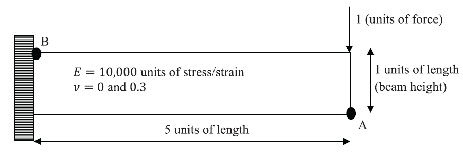
The shown triangular element has a thickness of  , and
, and  . Find the stiffness matrices in the plane stress and plane strain conditions. Also, find the displacements corresponding to the shown loading and boundary conditions in the case of plane strain. Compare with the solution obtained using ABAQUS.
SOLUTION
The isoparametric triangle element has the following shape functions:
![\[N_1 = 1 - \xi - \eta\]](https://engcourses-uofa.ca/wp-content/ql-cache/quicklatex.com-1cc49ccdea1a3f45b7f2126424b7211c_l3.png "Rendered by QuickLaTeX.com")
![\[N_2 = \xi\]](https://engcourses-uofa.ca/wp-content/ql-cache/quicklatex.com-ae4646f9754fd5ec8c0f94841c042c9f_l3.png "Rendered by QuickLaTeX.com")
![\[N_3 = \eta\]](https://engcourses-uofa.ca/wp-content/ql-cache/quicklatex.com-7ae2d40de290e9084d35f28d68654e5a_l3.png "Rendered by QuickLaTeX.com")
The mapping functions between the spatial and element coordinate systems are given by:
![\[x = N_1x_1 + N_2x_2 + N_3x_3 = 2\eta + 5\xi\]](https://engcourses-uofa.ca/wp-content/ql-cache/quicklatex.com-6e71e73ff948cd8144526f38100bf193_l3.png "Rendered by QuickLaTeX.com")
![\[y = N_1y_1 + N_2y_2 + N_3y_3 = 6\eta\]](https://engcourses-uofa.ca/wp-content/ql-cache/quicklatex.com-b7326d9fae69a20961d725492390a0fe_l3.png "Rendered by QuickLaTeX.com")
The Jacobian of the transformation and its inverse are given by:
![\[J = \begin{pmatrix} \frac{\partial x}{\partial \xi} & \frac{\partial x}{\partial \eta} \\ \frac{\partial y}{\partial \xi} & \frac{\partial y}{\partial \eta} \\ \end{pmatrix} = \begin{pmatrix} 5 & 2 \\ 0 & 6 \\ \end{pmatrix}\]](https://engcourses-uofa.ca/wp-content/ql-cache/quicklatex.com-1011ba90ce4332937962e9fb23cad5b0_l3.png "Rendered by QuickLaTeX.com")
![\[J^{-1} = \begin{pmatrix} \frac{\partial \xi}{\partial x} & \frac{\partial \xi}{\partial y} \\ \frac{\partial \eta}{\partial x} & \frac{\partial \eta}{\partial y} \\ \end{pmatrix} = \begin{pmatrix} \frac{1}{5} & \frac{-1}{15} \\ 0 & \frac{1}{6} \end{pmatrix}\]](https://engcourses-uofa.ca/wp-content/ql-cache/quicklatex.com-a76cbeb546e9a64570e0b2c3714063c3_l3.png "Rendered by QuickLaTeX.com")
and  . The matrix
  with:
with:
![\[M_1 = \begin{pmatrix} 1 & 0 & 0 & 0 \\ 0 & 0 & 0 & 1 \\ 0 & 1 & 1 & 0 \\ \end{pmatrix}\]](https://engcourses-uofa.ca/wp-content/ql-cache/quicklatex.com-36836ae3e3f537270ceec2062194866f_l3.png "Rendered by QuickLaTeX.com")
![\[M_2 = \begin{pmatrix} \frac{\partial \xi}{\partial x} & \frac{\partial \xi}{\partial y} & 0 & 0 \\ \frac{\partial \eta}{\partial x} & \frac{\partial \eta}{\partial y} & 0 & 0 \\ 0 & 0 & \frac{\partial \xi}{\partial x} & \frac{\partial \eta}{\partial x} \\ 0 & 0 & \frac{\partial \xi}{\partial y} & \frac{\partial \eta}{\partial y} \\ \end{pmatrix} = \begin{pmatrix} \frac{1}{5} & 0 & 0 & 0 \\ \frac{-1}{15} & \frac{1}{6} & 0 & 0 \\ 0 & 0 & \frac{1}{5} & 0 \\ 0 & 0 & \frac{-1}{15} & \frac{1}{6} \\ \end{pmatrix}\]](https://engcourses-uofa.ca/wp-content/ql-cache/quicklatex.com-28f1338a7ab9ce493569d6ec5bd2b66d_l3.png "Rendered by QuickLaTeX.com")
![\[M_3 = \begin{pmatrix} \frac{\partial N_1}{\partial \xi} & 0 & \frac{\partial N_2}{\partial \xi} & 0 & \frac{\partial N_3}{\partial \xi} & 0 \\ \frac{\partial N_1}{\partial \eta} & 0 & \frac{\partial N_2}{\partial \eta} & 0 & \frac{\partial N_3}{\partial \eta} & 0 \\ 0 & \frac{\partial N_1}{\partial \xi} & 0 & \frac{\partial N_2}{\partial \xi} & 0 & \frac{\partial N_3}{\partial \xi} \\ 0 & \frac{\partial N_1}{\partial \eta} & 0 & \frac{\partial N_2}{\partial \eta} & 0 & \frac{\partial N_3}{\partial \eta} \\ \end{pmatrix}\]](https://engcourses-uofa.ca/wp-content/ql-cache/quicklatex.com-15ad0baddedfb9dbe68658e4c8707c1e_l3.png "Rendered by QuickLaTeX.com")
Therefore, the matrix is given by:
![\[B = \begin{pmatrix} \frac{-1}{5} & 0 & \frac{1}{5} & 0 & 0 & 0 \\ 0 & \frac{-1}{10} & 0 & \frac{-1}{15} & 0 & \frac{1}{6} \\ \frac{-1}{10} & \frac{-1}{5} & \frac{-1}{15} & \frac{1}{5} & \frac{1}{6} & 0 \\ \end{pmatrix}\]](https://engcourses-uofa.ca/wp-content/ql-cache/quicklatex.com-1fa7224b93fe38dc38ac73c07cf5539e_l3.png "Rendered by QuickLaTeX.com")
The stiffness matrix is given by:
![\[K = t \det{J} \int B^TCBdA\]](https://engcourses-uofa.ca/wp-content/ql-cache/quicklatex.com-c1b22123b8a68072318c005eb9908f8f_l3.png "Rendered by QuickLaTeX.com")
Full integration for both plane strain and plane stress conditions can be performed with one integration point with  ,
,  and the associated combined weight is
  .
.
![\[K = \frac{1}{2} t \det{J} B^TCB \Big|_{\xi = \frac{1}{3}, \eta = \frac{1}{3}}\]](https://engcourses-uofa.ca/wp-content/ql-cache/quicklatex.com-49e7c6bde90e4b4bf2074d376b6af16c_l3.png "Rendered by QuickLaTeX.com")
The following Mathematica code outputs the required stiffness matrices. The same stiffness matrices are obtained using ABAQUS. The columns of the stiffness matrix can be obtained using ABAQUS by restraining all the degrees of freedom to zero except for the degree of freedom corresponding to the desired column. The reactions obtained from ABAQUS are the columns of the stiffness matrix.
View Mathematica Code
nodes = {{0, 0}, {5, 0}, {2, 6}};
el1 = {1, 2, 3};
e1 = {nodes[[1]], nodes[[2]], nodes[[3]]};
Ee = 20000000000;
nu = 0.2;
Nn = {(1 - xi - eta), xi, eta};
(*Plane Stress*)
Cc2 = Ee/(1 + nu)*{{(1)/(1 - nu), nu/(1 - nu), 0}, {nu/(1 - nu), 1/(1 - nu), 0}, {0, 0, 1/2}};
(*Plane Strain*)
Cc1 = Ee/(1 + nu)*{{(1 - nu)/(1 - 2 nu), nu/(1 - 2 nu), 0}, {nu/(1 - 2 nu), (1 - nu)/(1 - 2 nu), 0}, {0, 0, 1/2}};
xe1 = Sum[Nn[[i]]*e1[[i, 1]], {i, 1, 3}]
ye1 = Sum[Nn[[i]]*e1[[i, 2]], {i, 1, 3}]
J1 = FullSimplify[{{D[xe1, xi], D[xe1, eta]}, {D[ye1, xi], D[ye1, eta]}}];
Jin1T = Transpose[Inverse[J1]];
J1 // MatrixForm
Jin1T // MatrixForm
JD1 = Det[J1];
Mat1 = {{1, 0, 0, 0}, {0, 0, 0, 1}, {0, 1, 1, 0}};
Mat2e1 = Table[0, {i, 1, 4}, {j, 1, 4}];
Mat2e1[[1 ;; 2, 1 ;; 2]] = Jin1T;
Mat2e1[[3 ;; 4, 3 ;; 4]] = Jin1T;
Mat3 = Table[0, {i, 1, 4}, {j, 1, 6}];
Do[Mat3[[1, 2 i - 1]] = Mat3[[3, 2 i]] = D[Nn[[i]], xi]; Mat3[[2, 2 i - 1]] = Mat3[[4, 2 i]] = D[Nn[[i]], eta], {i, 1, 3}];
B1 = Mat1.Mat2e1.Mat3;
B1 // MatrixForm
Kb2 = Transpose[B1].Cc1.B1;
Kb2 // MatrixForm;
K1 = JD1*Transpose[B1].Cc1.B1;
K1 // MatrixForm
Ki1 = 1/2*K1 /. {xi -> 1/3, eta -> 1/3};
Ki1 // MatrixForm
K2 = JD1*Transpose[B1].Cc2.B1;
K2 // MatrixForm
Ki2 = 1/2*K2 /. {xi -> 1/3, eta -> 1/3};
Ki2 // MatrixForm
(*In the following, nodes 1 and 2 are restrained in the plane strain condition and a horizontal load of 50,000,000N and vertical of -50,000,000N are applied on node 3*)
Kk = Ki1[[5 ;; 6, 5 ;; 6]];
Ff = Table[0, {i, 1, 2}];
Ff[[1]] = 50000000;
Ff[[2]] = -50000000;
Ff // MatrixForm
u = Inverse[Kk].Ff;
u // MatrixForm
ud = {0, 0, 0, 0, u[[1]], u[[2]]};
ud // MatrixForm
B1.ud // MatrixForm
View Python Code
from sympy import *
import sympy as sp
xi,eta = sp.symbols("xi eta")
nodes = [[0,0], [5,0], [2,6]]
el1 = Matrix([1,2,3])
e1 = Matrix([[0,0], [5,0], [2,6]])
E = 20000000000
nu = 0.2
Nn = Matrix([[1-xi-eta], [xi], [eta]])
display("Shape Functions: ", Nn)
Cc2 = E/(1+nu)*Matrix([[1/(1 - nu), nu/(1 - nu), 0],
                       [nu/(1 - nu), 1/(1 - nu), 0],
                       [0, 0, 1/2]])
display("Plane Stress: ", Cc2)
Cc1 = E/(1+nu)*Matrix([[(1 - nu)/(1 - 2 * nu), nu/(1 - 2 * nu), 0],
                       [nu/(1 - 2 * nu), (1 - nu)/(1 - 2 * nu), 0],
                       [0, 0, 1/2]])
display("Plane Strain: ", Cc1)
xe1 = sum(Nn[i] * e1[i,0] for i in range(3))
ye1 = sum(Nn[i] * e1[i,1] for i in range(3))
display("Mapping functions: ",xe1,ye1)
J1 = Matrix([[xe1.diff(xi), xe1.diff(eta)], [ye1.diff(xi), ye1.diff(eta)]])
display("Jacobian Transformation: ", J1)
lol = Inverse(J1)
J1in1t = J1.inv()
display("Inverse: ", J1in1t)
JD1 = J1.det()
display("Determinant: ", JD1)
Mat1 = Matrix([[1,0,0,0],[0,0,0,1],[0,1,1,0]])
Mat2 = Matrix([[J1in1t[0,0], J1in1t[1,0], 0, 0],
                 [J1in1t[0,1], J1in1t[1,1], 0, 0],
                 [0, 0, J1in1t[0,0], J1in1t[1,0]],
                 [0, 0, J1in1t[0,1], J1in1t[1,1]]])
Mat3 = Matrix([[Nn[0].diff(xi), 0, Nn[1].diff(xi), 0, Nn[2].diff(xi), 0],
               [Nn[0].diff(eta), 0, Nn[1].diff(eta), 0, Nn[2].diff(eta), 0],
               [0, Nn[0].diff(xi), 0, Nn[1].diff(xi), 0, Nn[2].diff(xi)],
               [0, Nn[0].diff(eta), 0, Nn[1].diff(eta), 0, Nn[2].diff(eta)]])
B = Mat1*Mat2*Mat3
display("B: ", B)
Kb2 = B.transpose()*Cc1*B
K1 = JD1*Kb2
Ki1 = sympify(1/2)*K1
K2 = JD1*B.transpose()*Cc2*B
Ki2 = 1/2*K2
K = Matrix([[Ki1[4,4], Ki1[4,5]],[Ki1[5,4], Ki1[5,5]]])
F = Matrix([50000000, -50000000])
u = K.inv()*F
ud = Matrix([0,0,0,0,u[0],u[1]])
display("strain: ", B*ud)
Under the applied load, in the plane strain condition, the horizontal displacement  and vertical displacement
  of the top node can be obtained by reducing the equations (eliminating the rows and columns corresponding to degrees of freedom
  ) as follows:
![\[\begin{pmatrix} K_{55} & K_{56} \\ K_{56} & K_{66} \\ \end{pmatrix} \begin{pmatrix} u_3 \\ v_3 \\ \end{pmatrix} = \begin{pmatrix} 50000000 \\ -50000000 \\ \end{pmatrix}\]](https://engcourses-uofa.ca/wp-content/ql-cache/quicklatex.com-f214d2efa298e5534b5b6d54105d30b7_l3.png "Rendered by QuickLaTeX.com")
Therefore,  , and
, and  . The corresponding strain in the element can be obtained as follows:
![\[\begin{pmatrix} \varepsilon_{xx} \\ \varepsilon_{yy} \\ \gamma_{xy} \\ \end{pmatrix} = B \begin{pmatrix} u_1 \\ v_1 \\ u_2 \\ v_2 \\ u_3 \\ v_3 \\ \end{pmatrix}\]](https://engcourses-uofa.ca/wp-content/ql-cache/quicklatex.com-0fbf882abfc767e17829f7e1ad8c9f06_l3.png "Rendered by QuickLaTeX.com")
![\[= \begin{pmatrix} \frac{-1}{5} & 0 & \frac{1}{5} & 0 & 0 & 0 \\ 0 & \frac{-1}{10} & 0 & \frac{-1}{15} & 0 & \frac{1}{6} \\ \frac{-1}{10} & \frac{-1}{5} & \frac{-1}{15} & \frac{1}{5} & \frac{1}{6} & 0 \\ \end{pmatrix} \begin{pmatrix} 0 \\ 0 \\ 0 \\ 0 \\ 0.0144 \\ -0.0054 \\ \end{pmatrix}\]](https://engcourses-uofa.ca/wp-content/ql-cache/quicklatex.com-d7702ce3a4c5bf1b3447c692a366e7ae_l3.png "Rendered by QuickLaTeX.com")
![\[= \begin{pmatrix} 0 \\ -0.0009 \\ 0.0024 \\ \end{pmatrix}\]](https://engcourses-uofa.ca/wp-content/ql-cache/quicklatex.com-3ac6db0f43ccf4e07248d70f511c12e1_l3.png "Rendered by QuickLaTeX.com")
The same exact results for the three strains are obtained using ABAQUS (version 6.12)


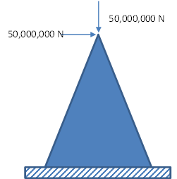
Example 3
Consider the shown structure (Plane strain) with  ,
,  under the shown concentrated load. Using two triangular elements, find the displacement of the top nodes.
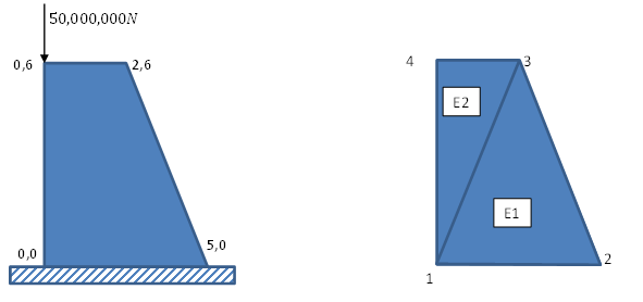
SOLUTION
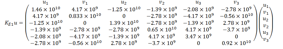
Following the procedure in the previous example, element E1 has the following stiffness matrix with the corresponding degrees of freedom:
Element E2 has the following stiffness matrix with the corresponding degrees of freedom:
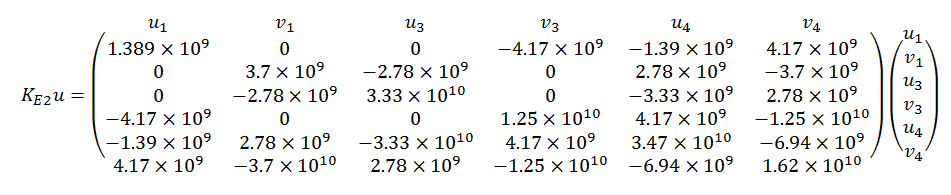
The global stiffness matrix is an  matrix with the following entries and corresponding degrees of freedom:
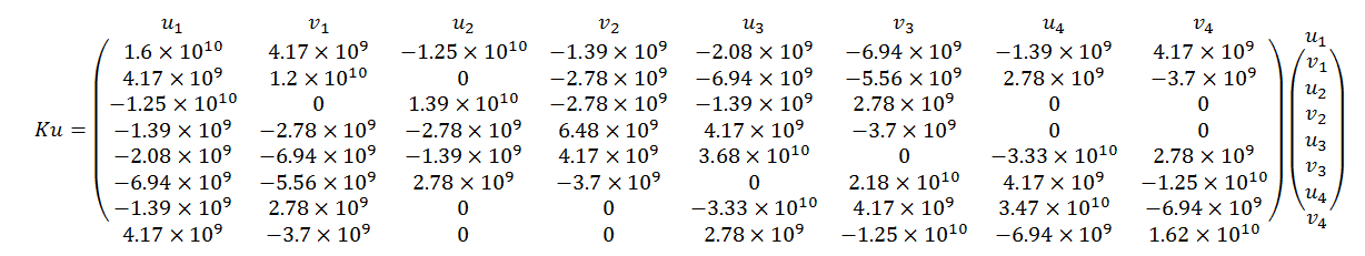
By reducing the matrix (removing the rows and columns corresponding to  ,
,  , , and
  , we are left with a
  matrix. The corresponding force vector is:
![\[f = \begin{pmatrix} 0 \\ 0 \\ 0 \\ -50,000,000 \\ \end{pmatrix}\]](https://engcourses-uofa.ca/wp-content/ql-cache/quicklatex.com-28852d928e285bcbc9c2b798dad62365_l3.png "Rendered by QuickLaTeX.com")
The corresponding displacements (in m.) are:
![\[u = \begin{pmatrix} u_3 \\ v_3 \\ u_4 \\ v_4 \\ \end{pmatrix} = \begin{pmatrix} -0.0027 \\ -0.0031 \\ -0.0035 \\ -0.0065 \\ \end{pmatrix}\]](https://engcourses-uofa.ca/wp-content/ql-cache/quicklatex.com-fc11b46b0b448e3db8c8b34513b1efaf_l3.png "Rendered by QuickLaTeX.com")
The following is the Mathematica code utilized. The variables mape1 and mape2 were used to map the local degrees of freedom of elements 1 and 2 respectively to the global degrees of freedom for the global matrix assembly.
View Mathematica Code
nodes = {{0, 0}, {5, 0}, {2, 6}, {0, 6}};
el1 = {1, 2, 3};
el2 = {1, 3, 4};
e1 = {nodes[[1]], nodes[[2]], nodes[[3]]};
e2 = {nodes[[1]], nodes[[3]], nodes[[4]]};
mape1 = {2*el1[[1]] - 1, 2*el1[[1]], 2*el1[[2]] - 1, 2*el1[[2]], 2*el1[[3]] - 1, 2*el1[[3]]};
mape2 = {2*el2[[1]] - 1, 2*el2[[1]], 2*el2[[2]] - 1, 2*el2[[2]], 2*el2[[3]] - 1, 2*el2[[3]]};
mape1 // MatrixForm
mape2 // MatrixForm
Ee = 20000000000;
nu = 0.2;
Nn = {(1 - xi - eta), xi, eta};
(*Plane Strain*)
Cc1 = Ee/(1 + nu)*{{(1 - nu)/(1 - 2 nu), nu/(1 - 2 nu), 0}, {nu/(1 - 2 nu), (1 - nu)/(1 - 2 nu), 0}, {0, 0, 1/2}};
(*Element 1*)
xe1 = Sum[Nn[[i]]*e1[[i, 1]], {i, 1, 3}]
ye1 = Sum[Nn[[i]]*e1[[i, 2]], {i, 1, 3}]
J1 = FullSimplify[{{D[xe1, xi], D[xe1, eta]}, {D[ye1, xi], D[ye1, eta]}}];
Jin1T = Transpose[Inverse[J1]];
JD1 = Det[J1];
Mat1 = {{1, 0, 0, 0}, {0, 0, 0, 1}, {0, 1, 1, 0}};
Mat2e1 = Table[0, {i, 1, 4}, {j, 1, 4}];
Mat2e1[[1 ;; 2, 1 ;; 2]] = Jin1T;
Mat2e1[[3 ;; 4, 3 ;; 4]] = Jin1T;
Mat3 = Table[0, {i, 1, 4}, {j, 1, 6}];
Do[Mat3[[1, 2 i - 1]] = Mat3[[3, 2 i]] = D[Nn[[i]], xi]; Mat3[[2, 2 i - 1]] = Mat3[[4, 2 i]] = D[Nn[[i]], eta], {i, 1, 3}];
B1 = Mat1.Mat2e1.Mat3;
B1 // MatrixForm
Kb2 = Transpose[B1].Cc1.B1;
Kb2 // MatrixForm;
K1 = JD1*Transpose[B1].Cc1.B1;
K1 // MatrixForm;
Ki1 = 1/2*K1 /. {xi -> 1/3, eta -> 1/3};
Ki1 // MatrixForm
(*Element 2*)
xe2 = Sum[Nn[[i]]*e2[[i, 1]], {i, 1, 3}]
ye2 = Sum[Nn[[i]]*e2[[i, 2]], {i, 1, 3}]
J2 = FullSimplify[{{D[xe2, xi], D[xe2, eta]}, {D[ye2, xi], D[ye2, eta]}}];
Jin2T = Transpose[Inverse[J2]];
JD2 = Det[J2];
Mat1 = {{1, 0, 0, 0}, {0, 0, 0, 1}, {0, 1, 1, 0}};
Mat2e2 = Table[0, {i, 1, 4}, {j, 1, 4}];
Mat2e2[[1 ;; 2, 1 ;; 2]] = Jin2T;
Mat2e2[[3 ;; 4, 3 ;; 4]] = Jin2T;
Mat3 = Table[0, {i, 1, 4}, {j, 1, 6}];
Do[Mat3[[1, 2 i - 1]] = Mat3[[3, 2 i]] = D[Nn[[i]], xi]; Mat3[[2, 2 i - 1]] = Mat3[[4, 2 i]] = D[Nn[[i]], eta], {i, 1, 3}];
B2 = Mat1.Mat2e2.Mat3;
Kb2 = Transpose[B2].Cc1.B2;
Kb2 // MatrixForm;
K2 = JD2*Transpose[B2].Cc1.B2;
K2 // MatrixForm;
Ki2 = 1/2*K2 /. {xi -> 1/3, eta -> 1/3};
Ki2 // MatrixForm
Ktotal = Table[0, {i, 1, 8}, {j, 1, 8}];
Do[Ktotal[[mape1[[i]], mape1[[j]]]] = Ktotal[[mape1[[i]], mape1[[j]]]] + Ki1[[i, j]], {i, 1, 6}, {j, 1, 6}];
Do[Ktotal[[mape2[[i]], mape2[[j]]]] = Ktotal[[mape2[[i]], mape2[[j]]]] + Ki2[[i, j]], {i, 1, 6}, {j, 1, 6}];
Ktotal // MatrixForm
Kk = Ktotal[[5 ;; 8, 5 ;; 8]];
ff = {0, 0, 0, -50000000};
Inverse[Kk].ff // MatrixForm
View Python Code
import sympy as sp
from sympy import Matrix,diff
xi,eta = sp.symbols("xi eta")
nodes = [[0,0],[5,0],[2,6],[0,6]]
el1 = Matrix([1,2,3])
el2 = Matrix([1,3,4])
e1 = Matrix([nodes[0],nodes[1],nodes[2]])
e2 = Matrix([nodes[0],nodes[2],nodes[3]])
map1 = [2*el1[0]-1,2*el1[0],2*el1[1]-1,2*el1[1],2*el1[2]-1,2*el1[2]]
map2 = [2*el2[0]-1,2*el2[0],2*el2[1]-1,2*el2[1],2*el2[2]-1,2*el2[2]]
E = 20000000000
nu = 0.2
Nn = Matrix([[1-xi-eta],[xi],[eta]])
Cc1 = E/(1+nu)*Matrix([[(1-nu)/(1-2*nu),nu/(1-2*nu),0],
                       [nu/(1-2*nu),(1-nu)/(1-2*nu),0],
                       [0,0,1/2]])
display("Plane Strain: ", Cc1)
def calculate(e):
    xe = sum(Nn[i]*e[i,0] for i in range(3))
    ye = sum(Nn[i]*e[i,1] for i in range(3))
    display("Mapping functions =",xe,ye)
    J = Matrix([[xe.diff(xi), xe.diff(eta)], [ye.diff(xi), ye.diff(eta)]])
    display("Jacobian Transformation =", J)
    Jin1t = J.T.inv()
    display("Inverse =", Jin1t)
    JD = J.det()
    display("Determinant =", JD)
    Mat1 = Matrix([[1,0,0,0],[0,0,0,1],[0,1,1,0]])
    Mat2 = Matrix([[Jin1t[0,0], Jin1t[0,1],0,0],
                    [Jin1t[1,0],Jin1t[1,1],0,0],
                    [0,0,Jin1t[0,0],Jin1t[0,1]],
                    [0,0,Jin1t[1,0],Jin1t[1,1]]])
    Mat3 = Matrix([[Nn[0].diff(xi),0,Nn[1].diff(xi),0,Nn[2].diff(xi),0],
                   [Nn[0].diff(eta),0,Nn[1].diff(eta),0,Nn[2].diff(eta),0],
                   [0,Nn[0].diff(xi),0,Nn[1].diff(xi),0,Nn[2].diff(xi)],
                   [0,Nn[0].diff(eta),0,Nn[1].diff(eta),0,Nn[2].diff(eta)]])
    B = Mat1*Mat2*Mat3
    display("B =", B)
    Kb2 = B.T*Cc1*B
    K = JD*Kb2
    Ki = (1/2)*K
    display("Ki =",Ki)
    return Ki
display("Element E1")
Ki1 = calculate(e1)
display("Element E2")
Ki2 = calculate(e2)
ktotal = Matrix([[0 for x in range(8)] for y in range(8)])
for i in range(6):
    for j in range(6):
        i1,j1 = map1[i]-1,map1[j]-1
        i2,j2 = map2[i]-1,map2[j]-1
        ktotal[i1,j1] = ktotal[i1,j1]+Ki1[i,j]
        ktotal[i2,j2] = ktotal[i2,j2]+Ki2[i,j]
display("ktotal =",ktotal)
Kk = Matrix(ktotal[4:8,4:8])
display(Kk)
ff = Matrix([0,0,0,-50000000])
display("Force vector =",ff)
u = Kk.inv()*ff
display("Displacements =",u)
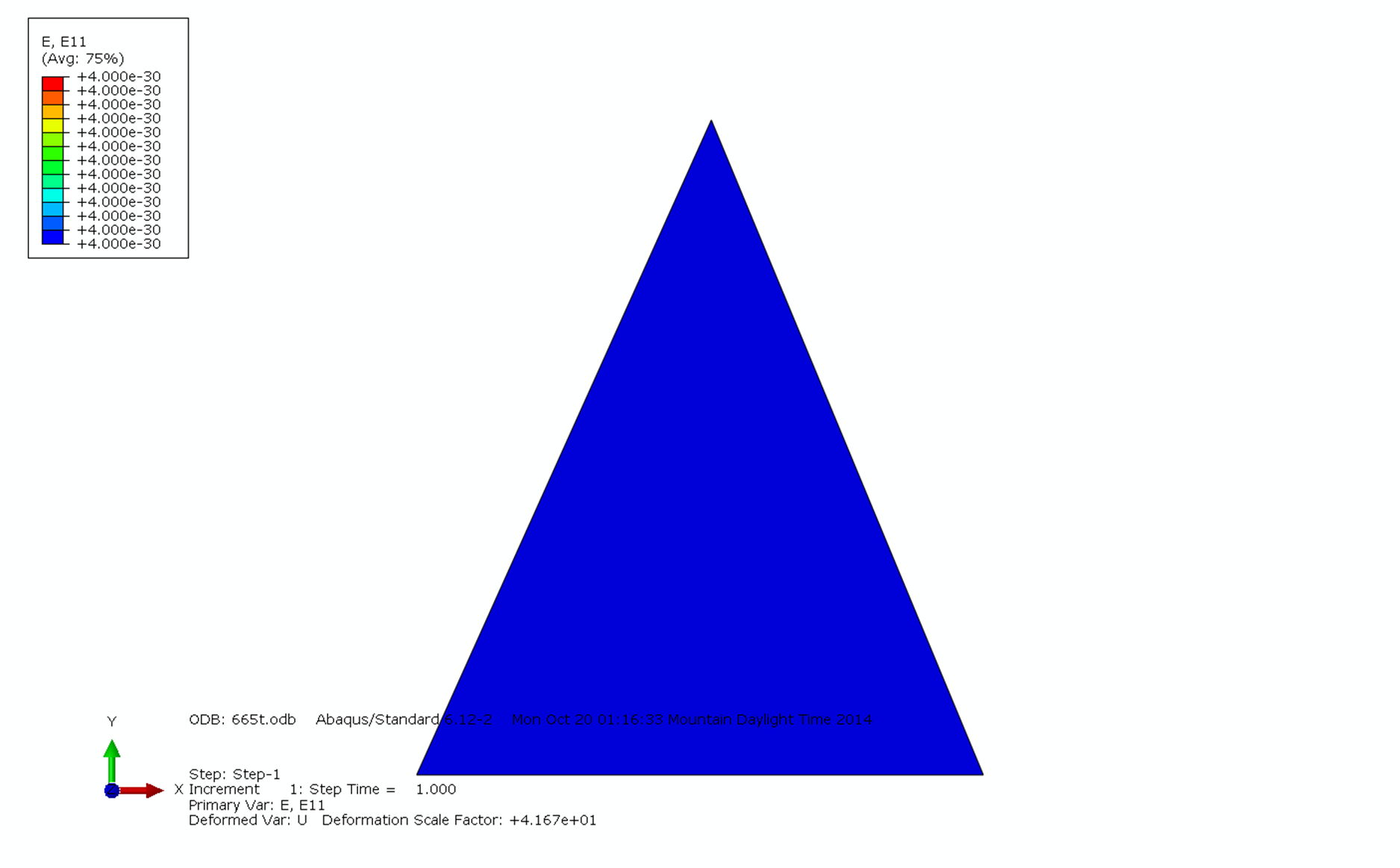
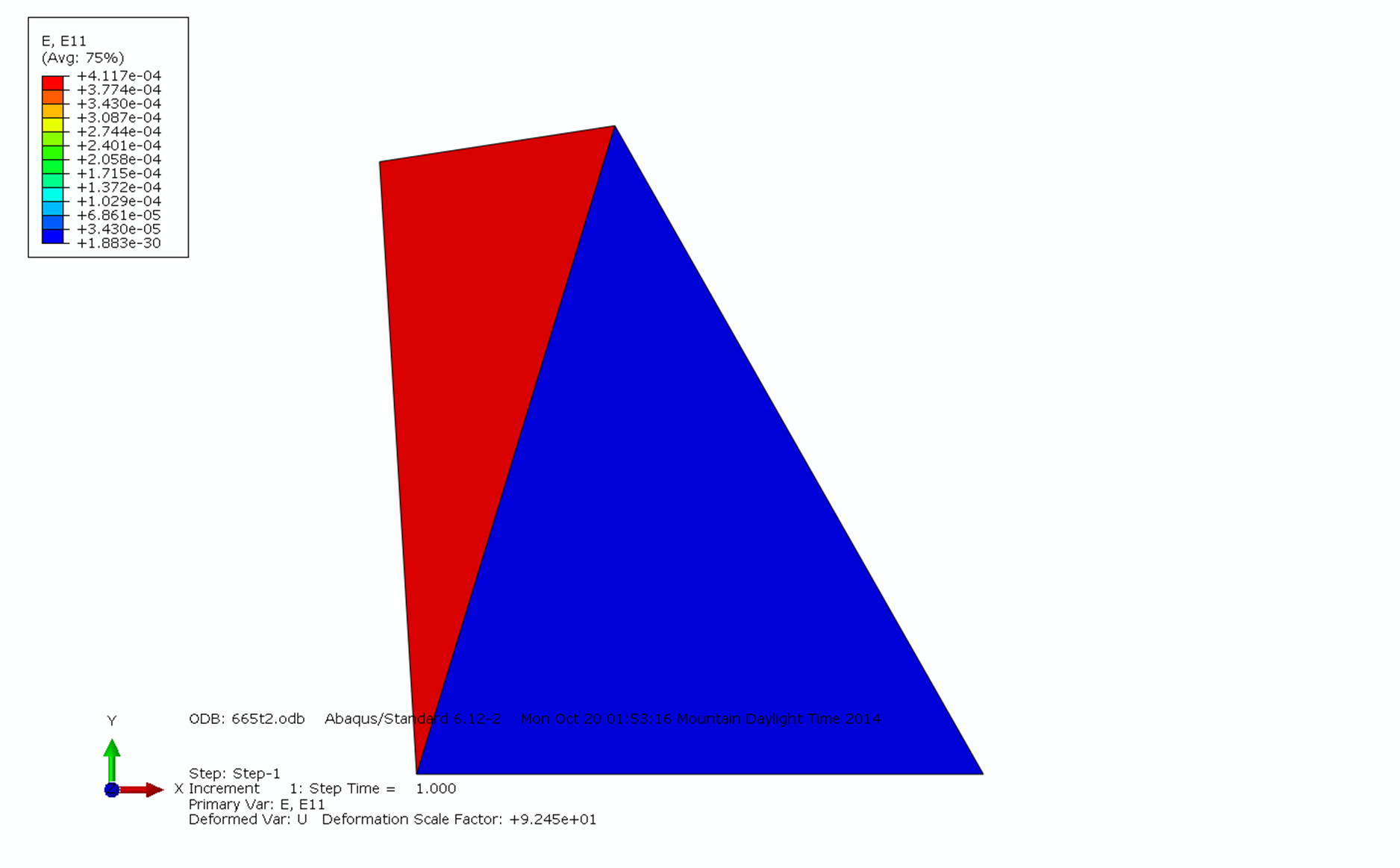
ABAQUS results are exactly the same for this element. Below is the output from ABAQUS (version 6.12) showing the discontinuity in the longitudinal strain component  .
.
Problems
A plane element has length of 2 units aligned with the
 axis and height of 4 units that is aligned with the
  axis. If a pure rigid-body rotation around the z (out of plane) axis of angle
  is applied to the element, find the corresponding variation in the magnitude of the small “apparent” strain components. Then, use a finite element analysis software to compare your theoretical results with the software results by assigning different values for . Comment on the results. Then, if the software used has a geometric non-linearity option, inspect the effect of selecting this option on the magnitudes of the resulting strain components at the different chosen values for . (Hint: the rotation of the element can be applied by directly applying the appropriate displacements to the corner nodes.)
Using any finite element analysis software of your choice, find the deflection at point A and the stress components at point B as a function of the number of elements used per the height of the beam. Use 4-node quadrilateral full integration elements. Compare with the Euler-Bernoulli beam solution. Solve twice, once with Poisson’s ratio = 0 and another time with Poisson’s ratio = 0.3. Consider the thickness to be 1 units of length.
Solve the previous problem using reduced integration 4-node elements and reduced integration 8-node elements. Compare with the results obtained in the previous problem. Comment on the convergence rate. Comment also on whether all the elements are converging to the same solution or not.
Use a suitable quadrature to evaluate the following integrals and compare with the exact solution. Comment on the results in reference to the finite element analysis method integration scheme.

Find the Jacobian matrix for a 4-node quadrilateral isoparametric element whose coordinates are: (1,1), (3,2), (4,4), and (2,5). Assuming plane strain, unit thickness, and
 , find the stiffness matrix using (a) the built-in integration function in Mathematica, (b) full Gauss integration scheme, and (c) reduced Gauss integration scheme
Following Example 1 above, use different element shapes to comment on the following.
The effect of increasing the distortion of the element on
 and
and  before integration.
The effect of increasing the distortion of the element on the difference between
and for the exact integration, full integration, and reduced integration schemes.If the isoparametric element is rectangular in shape but is rotated in space, what is the effect of the angle of rotation on
and in the case of exact integration, full integration, and reduced integration schemes.
The following are two main requirements for the shape functions of a 4-node quadrilateral element that has a general non-rectangular shape:
The sum of all the shape functions has to be equal to unity to ensure that rigid body motion is feasible.
The displacement of the element side is fully determined only by the displacement of the nodes to which this side is connected in a manner that ensures element compatibility.>
Does the isoparametric element formulation of a general element shape ensure the above requirements? Show that one or both of those requirements are not met if in Example 1 above either of the following two methods was used to find the shape functions:
Method 1: By assuming the following bilinear displacement across the element:


Method 2: By assuming that the shape function of each node is equal to 1 at the specified node and zero on the two sides not connected to that node
The shown structure has
 and is subjected to the shown pressure. Assume that the structure has a unit thickness of
  .
.Solve the closed form solution of the differential equation of equilibrium assuming the only unknowns are the vertical displacements and the corresponding normal stresses ignoring the effect of Poisson’s ratio.
Compare the solution using a finite element analysis software using
and  .
.
The shown two dimensional plane strain linear elastic three node triangular element has two side lengths equal to 2m.
 , and . One of the sides is loaded with a trapezoidal load as shown in the figure.
Find the
matrix and the stiffness matrix.Find the nodal forces vector.
If the nodal displacements of nodes 1, 2, and 3 of the element are given by (23,10), (0,30), and (20,0), respectively (units of mm), find the three-dimensional strain and stress components at
 .
.
Displacement finite element analyses are used to obtain the response of a structure to the applied external loading. For such problems, the term “linear” is used to designate “linear elements” and “linear response”. Briefly, explain the difference between “linear elements” and “linear response”. Give examples to justify your answer.
Calculate the stiffness matrix of the 8 node reduced integration plane quadrilateral element. Using the calculated stiffness matrix, calculate the nodal forces vector associated with its spurious mode.