Engineering at Alberta Courses » Videos, Examples, and Problems

Hyperelastic Materials: Videos, Examples, and Problems

Hyperelastic Materials Video

Examples

Example 1

Assume that a unit length cube of material deforms such that the length of the sides parallel to $e_1, e_2$ and $e_3$ become 0.8, 0.625 and l units, respectively, without any rotations. If the material follows a Neo-Hookean material model with $\mu=1$ units, find $l,W,\overline{U}$ , the Cauchy stress tensor $\sigma$ and the first Piola Kirchhoff stress tensor $P$ after deformation in terms of the unknown hydrostatic pressure $p$ .

SOLUTION

The deformation gradient of the above deformation is:

$F=\left(\begin{array}{ccc} 0.8 & 0 & 0\\ 0 & 0.625 & 0\\ 0 & 0 & l \end{array} \right)$

The material is incompressible, therefore $\det{F}F=1\Rightarrow l=2$ units. The first invariant of $U^2$ is given by:

$I_1 (U^2)=\lambda_1^2+\lambda_2^2+\lambda_3^2=0.8^2+0.625^2+2^2=5.03$

The strain energy per unit volume of the undeformed configuration is:

$W=2\mu(I_1 (U^2 )-3)=4.06 units$

Since $J=1\Rightarrow \overline{U}=W$ .
The stress matrices can be obtained by direct substitution in the equations for the stress:

$P=4\mu F+JpF^{-T}= \left(\begin{array}{ccc} 3.2+1.25p & 0 & 0\\ 0 & 2.5+1.6p & 0\\ 0 & 0 & 8+\frac{p}{2} \end{array} \right)$

$\sigma=4\mu FF^T+pI= \left(\begin{array}{ccc} 2.56+p & 0 & 0\\ 0 & 1.5625+p & 0\\ 0 & 0 & 16+p \end{array} \right)$

View Mathematica Code

F = {{0.8, 0, 0}, {0, 0.625, 0}, {0, 0, 2}};
J=Det[F];
mu=1;
I1=Sum[(Transpose[F].F)[[i,i]],{i,1,3}];
P=4*mu*F+J*p*Transpose[Inverse[F]];
sigma=4*mu*F.Transpose[F]+p*IdentityMatrix[3];
P//MatrixForm
sigma//MatrixForm

View Python Code

import sympy as sp
from sympy import *
F = Matrix([[0.8, 0, 0],[0, 0.625, 0],[0,0,2]])
J = det(F)
mu = 1
p = sp.symbols("p")
display("J = det(F) =",J)
display("F =",F)
I = sum(F*F.T)
display("I = sum(FF^T)",I)
P = 4*mu*F+J*p*F.inv().T
display("P = 4\u03BCF + JpF^(-T) =",P)
s = 4*mu*F*F.T+p*eye(3)
display("\u03C3 = 4\u03BCFFF^T+pI =",s)

Example 2

Assume that a unit length cube of material deforms such that the deformation gradient is:

$F=\left(\begin{array}{ccc} \frac{1}{4} & -\frac{1}{2\sqrt{2}} & \frac{1}{4}\\ \frac{1}{4} & \frac{1}{2\sqrt{2}} & \frac{1}{4}\\ -2\sqrt{2} & 0 & 2\sqrt{2} \end{array} \right)$

If the material follows a Neo-Hookean material model with $\mu=1$ units, find $l,W,\overline{U}$ , the Cauchy stress tensor $\sigma$ and the first Piola Kirchhoff stress tensor $P$ after deformation in terms of the unknown hydrostatic pressure $p$ .

SOLUTION

The determinant of $F$ is equal to 1, therefore, the deformation is isochoric.

$I_1 (F^T F)=33/2$

Both values of the strain energy per unit volume in the undeformed and the deformed configurations are equal:

$W=\overline{U}=2\mu(I_1 (F^T F)-3)=27units$

The stress matrices can be obtained by direct substitution in the equations for the stress:

$P=4\mu F+JpF^{-T}= \left(\begin{array}{ccc} 1+p & -\sqrt{2}(1+p) & 1+p\\ 1+p & \sqrt{2}(1+p) & 1+p\\ -8\sqrt{2}-\frac{p}{4\sqrt{2}} & 0 & 8\sqrt{2}+\frac{p}{4\sqrt{2}} \end{array} \right)$

$\sigma=4\mu FF^T+pI= \left(\begin{array}{ccc} 1+p & 0 & 0\\ 0 & 1+p & 0\\ 0 & 0 & 64+p \end{array} \right)$

View Mathematica Code

F = {{1/4, -1/2/Sqrt[2], 1/4}, {1/4, 1/2/Sqrt[2], 1/4}, {-2*Sqrt[2], 
   0, 2 Sqrt[2]}}
J = Det[F]
mu = 1
I1 = Sum[(Transpose[F] . F)[[i, i]], {i, 1, 3}]
P = 4*mu*F + J*p*Transpose[Inverse[F]];
sigma = 4*mu*F . Transpose[F] + p*IdentityMatrix[3];
P // MatrixForm
sigma // MatrixForm

View Python Code

import sympy as sp
from sympy import *
F = Matrix([[1/4,-1/(2*sp.sqrt(2)),1/4],
           [1/4,1/(2*sp.sqrt(2)),1/4],
           [-2*sp.sqrt(2),0,2*sp.sqrt(2)]])
J = det(F)
mu = 1
p = sp.symbols("p")
display("J = det(F) =",J)
display("F =",F)
I = sum(F*F.T)
display("I = sum(FF^T)",I)
P = 4*mu*F+J*p*F.inv().T
display("P = 4\u03BCF + JpF^(-T) =",P)
s = 4*mu*F*F.T+p*eye(3)
display("\u03C3 = 4\u03BCFFF^T+pI =",s)

Example 3

Draw the relationships between the components $P_{11}$ and $\sigma_{11}$ of the first Piola Kirchhoff stress tensor and the Cauchy stress tensor, respectively, versus $\lambda_1-1$ in a uniaxial state of stress using the three material models (Linear Elastic, Compressible Neo-Hookean, and compressible Mooney-Rivlin material (assuming $C_{10}=C_{01}$ )). Assume that the material is isotropic and no rotations occur during deformation. Assume two cases such that in the first case, in small deformations, the equivalent Young’s modulus and Poisson’s ratio are $E=20,000MPa$ and $\nu=0.49$ respectively. In the second case, in small deformations, the equivalent Young’s modulus and Poisson’s ratio are $E=20,000MPa$ and $\nu=0.2$ respectively.

SOLUTION

Because of the isotropy of the material, we can assume the following form for $F$ :

$F= \left(\begin{array}{ccc} \lambda_1 & 0 & 0\\ 0 & \lambda_2 & 0\\ 0 & 0 & \lambda_2 \end{array} \right)$

therefore $J=\lambda_1\lambda_2^2$ and

$F^{-T}= \left(\begin{array}{ccc} \frac{1}{\lambda_1} & 0 & 0\\ 0 & \frac{1}{\lambda_2} & 0\\ 0 & 0 & \frac{1}{\lambda_2} \end{array} \right)$

Linear Elastic Material:
For a linear elastic isotropic material,

$\varepsilon= \left(\begin{array}{ccc} \lambda_1-1 & 0 & 0\\ 0 & \lambda_2-1 & 0\\ 0 & 0 & \lambda_2-1 \end{array} \right)$

and therefore:

$\sigma=\frac{E}{(1-2\nu)(1+\nu)} \left(\begin{array}{ccc} \lambda_1(1-\nu)+2\nu\lambda_2-(1+\nu) & 0 & 0\\ 0 & \lambda_2+\nu\lambda_1-(1+\nu) & 0\\ 0 & 0 & \lambda_2+\nu\lambda_1-(1+\nu) \end{array} \right)$

Since it is a uniaxial state of stress, we have $\sigma_{22}=\sigma_{33}=0$ , therefore, $\lambda_2=-\nu\lambda_1+(1+\nu)$
Then:

$\sigma=E \left(\begin{array}{ccc} \lambda_1-1 & 0 & 0\\ 0 & 0 & 0\\ 0 & 0 & 0 \end{array} \right)$

The first Piola Kirchhoff stress is:

$P=J\sigma F^{-T}=E(-\nu\lambda_1+1+\nu)^2 \left(\begin{array}{ccc} \lambda_1-1 & 0 & 0\\ 0 & 0 & 0\\ 0 & 0 & 0 \end{array} \right)$

Therefore, $P_{11}=E(\lambda_1-1) (-\nu\lambda_1+1+\nu)^2$

Compressible Neo-Hookean Material:
The strain energy function, the first Piola Kirchhoff stress tensor and the Cauchy stress tensor are given by:

$W=C_{10} \left(\overline{I_1}-3\right)+\frac{1}{D}(J-1)^2$

$P=C_{10} J^{-\frac{2}{3}} \left(2F-\frac{2I_1}{3} F^{-T}\right)+\frac{2}{D}(J-1)JF^{-T}$

$\sigma=C_{10} J^{-\frac{5}{3}} \left(2FF^T-\frac{2I_1}{3} I\right)+\frac{2}{D}(J-1)I$

Where $C_{10}$ and $D$ are material constants that can be calibrated as described above such that $C_{10}=\frac{G}{2}$ and $\frac{2}{D}=K$
The normal components of the Cauchy stress in the second and third directions are given by:

$\sigma_{33}=\sigma_{22}=C_{10} J^{-\frac{5}{3}} \left(2\lambda_2^2-\frac{2}{3} (\lambda_1^2+\lambda_2^2+\lambda_2^2)\right)+\frac{2}{D}(\lambda_1\lambda_2^2-1)$

Setting $\sigma_{22}=0$ we get a relationship between $\lambda_1$ and $\lambda_2$ which can be used to substitute for $\lambda_2$ . The equations can be solved numerically by first assuming a value for $\lambda_1$ , then solving for $\lambda_2$ and substituting in the expressions for $\sigma_{11}$ and $P_{11}$ .

For a Compressible Mooney-Rivlin Material:
The strain energy function, the first Piola Kirchhoff stress tensor and the Cauchy stress tensor are given by:

$W=C_{10}\left(\overline{I_1}-3\right)+C_{01}\left(\overline{I_2}-3\right)+\frac{1}{D}(J-1)^2$

$P=C_{10} J^{-\frac{2}{3}} \left(2F-\frac{2I_1}{3} F^{-T}\right) +C_{01}J^{-\frac{4}{3}} \left(2I_1F-2FF^TF-\frac{4I_2}{3} F^{-T}\right) +\frac{2}{D}(J-1)JF^{-T}$

$\sigma=C_{10} J^{-\frac{5}{3}} \left(2FF^T-\frac{2I_1}{3} I\right)+ C_{01}J^{-\frac{7}{3}} \left(2I_1FF^T-2FF^TFF^T-\frac{4I_2}{3} I\right) +\frac{2}{D}(J-1)I$

Where $C_{10}, C_{01}$ and $D$ are material constants and can be calibrated as shown above such that $C_{10}=C_{01}=\frac{G}{4}$ and $\frac{2}{D}=K$

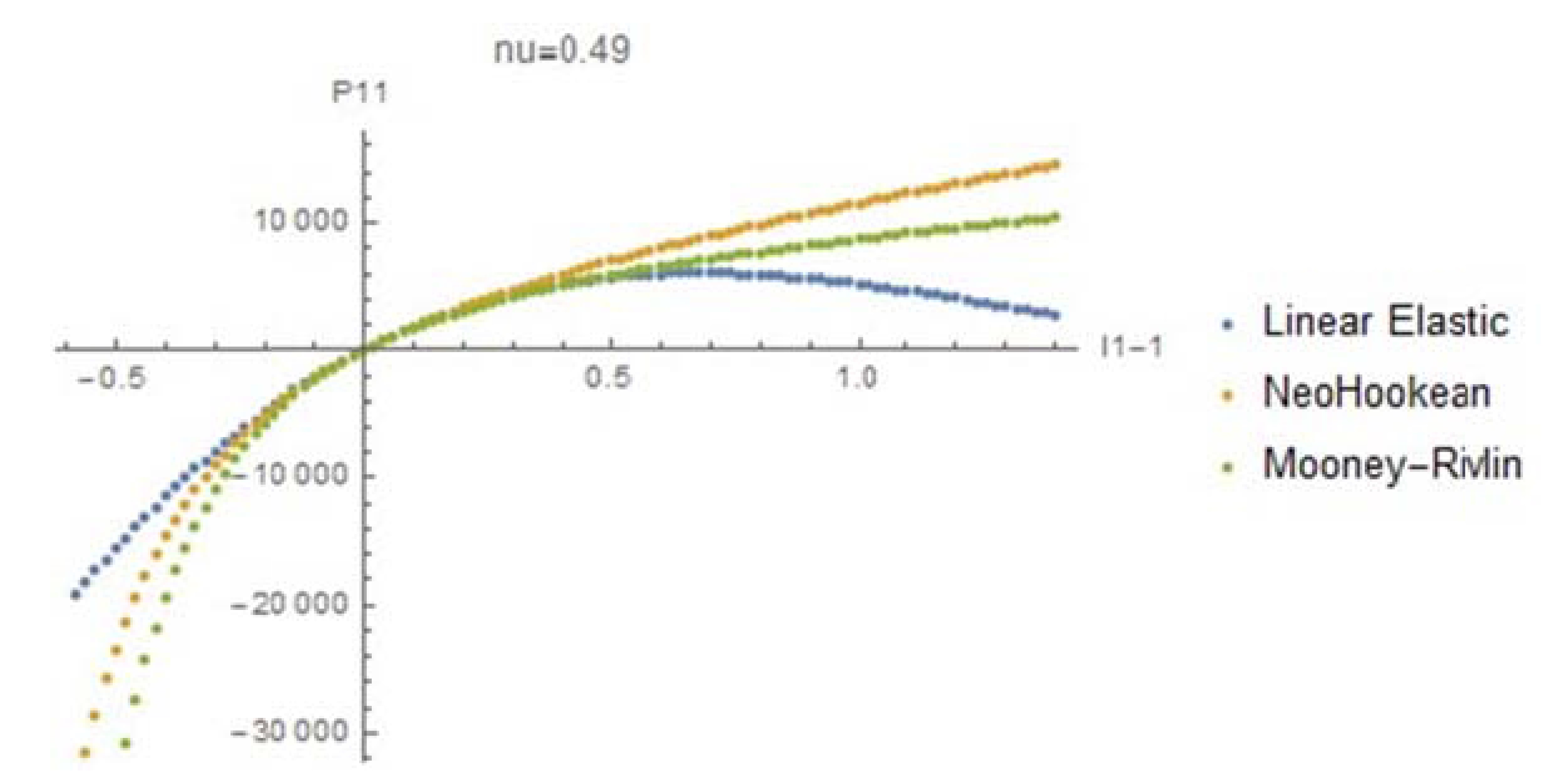
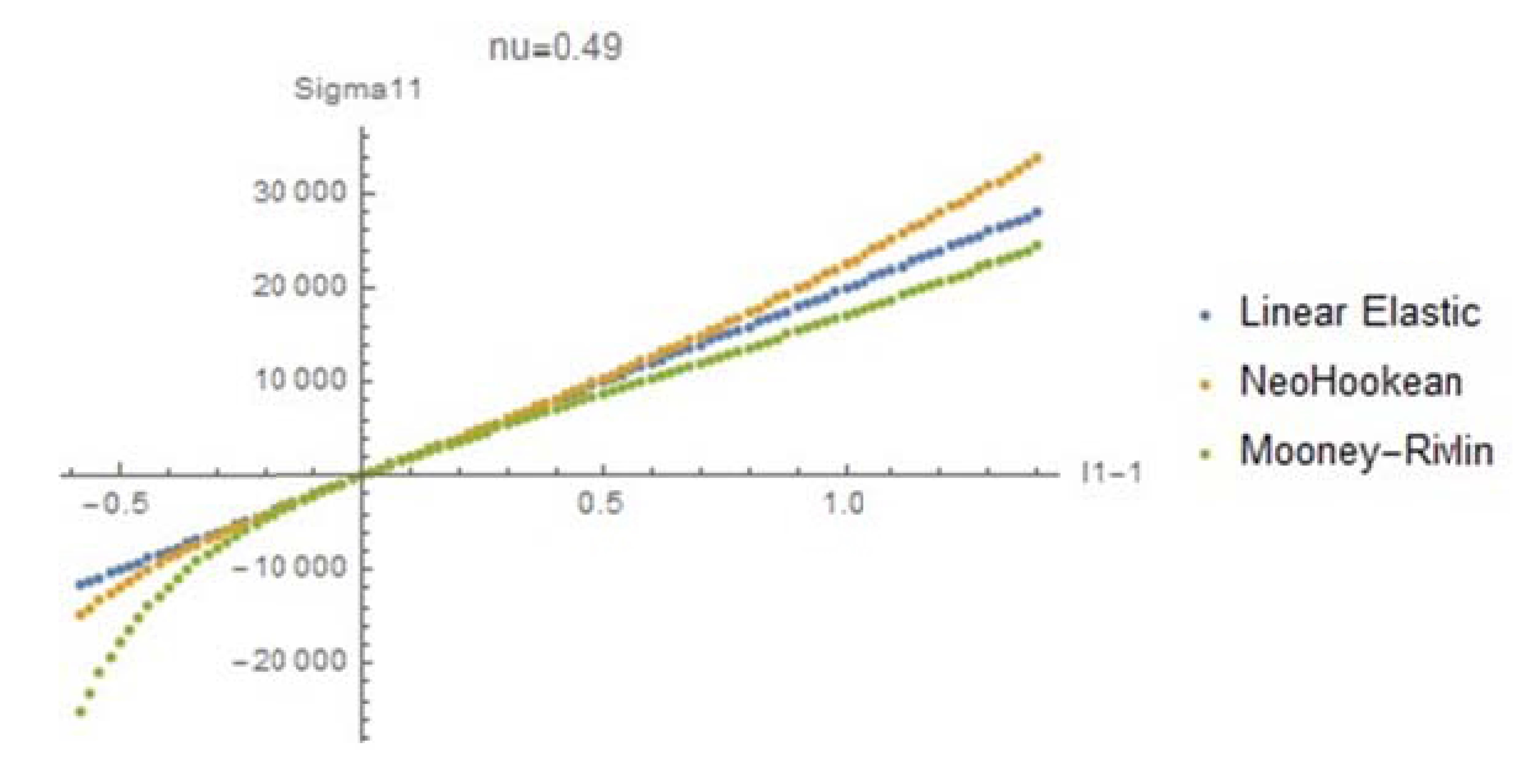
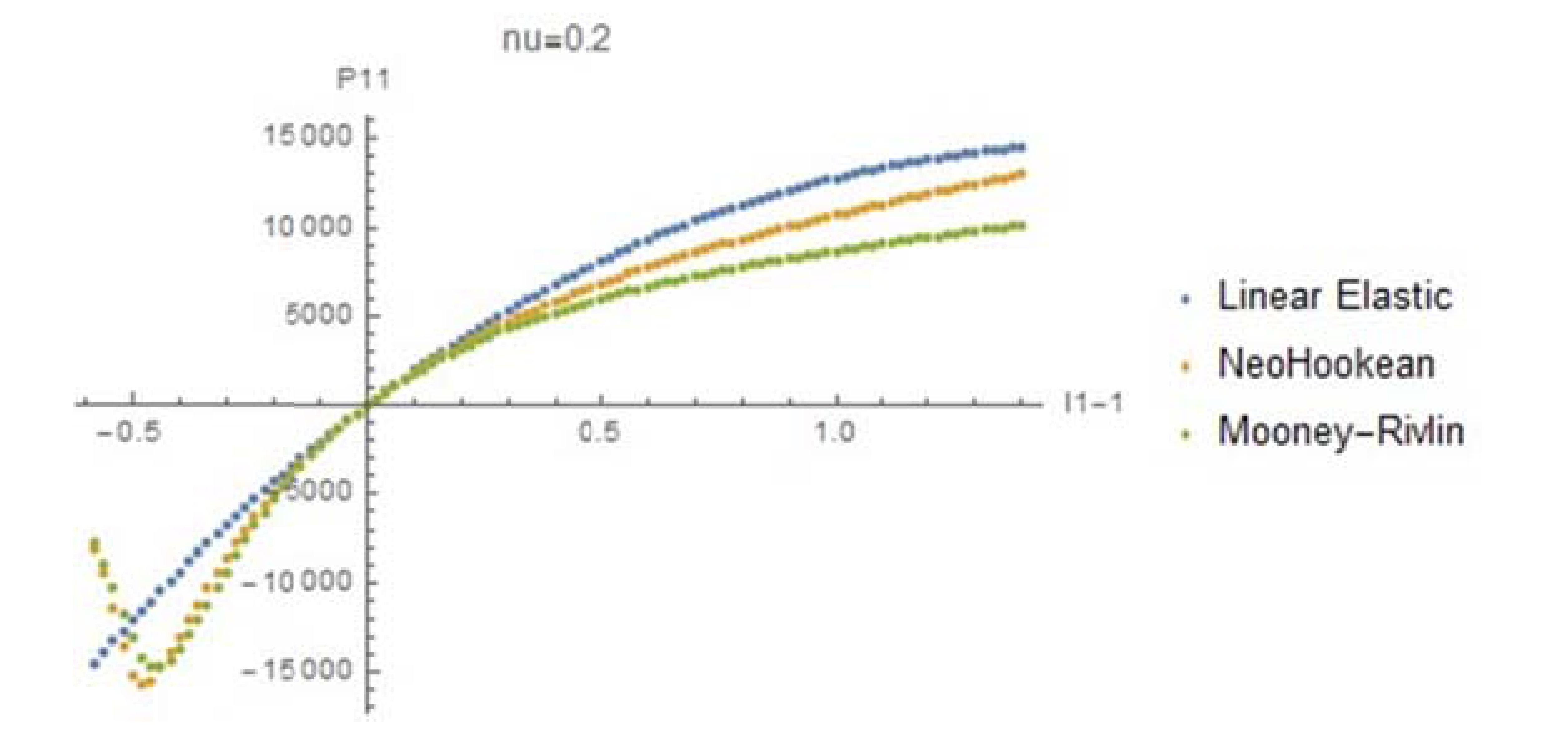
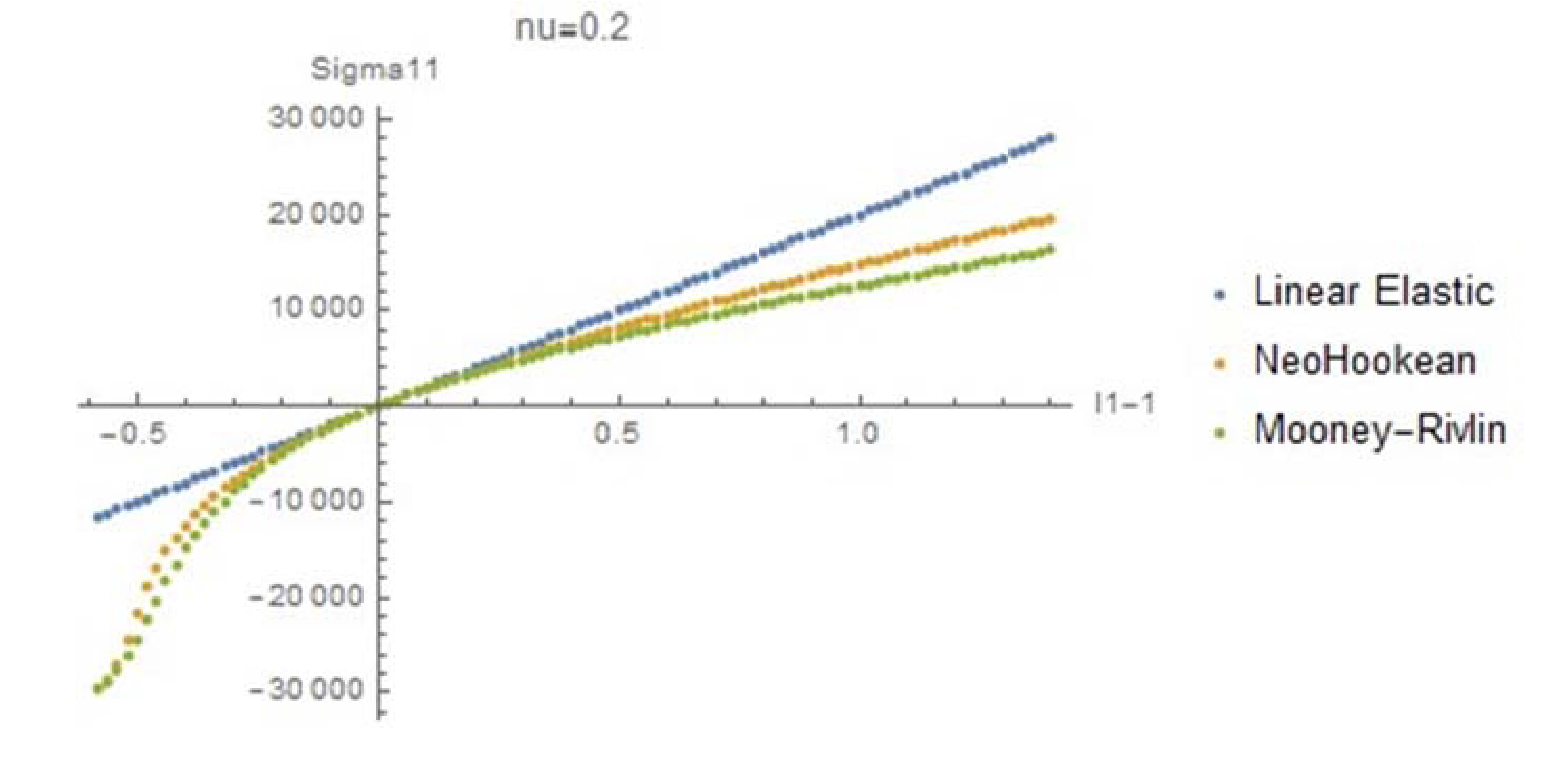
In the above relationship we have $\sigma_{33}=\sigma_{22}$ . Setting $\sigma_{22}=0$ we get a relationship between $\lambda_1$ and $\lambda_2$ which can be used to substitute for $\lambda_2$ . The equations can be solved numerically by first assuming a value for $\lambda_1$ , then solving for $\lambda_2$ and substituting in the expressions for $\sigma_{11}$ and $P_{11}$ . The required plots are shown below with MPa units for the stresses. Note the following, for $\nu=0.49$ , the first Piola Kirchhoff stress tensor component $P_{11}$ starts decreasing after $\lambda_1-1$ reaches around 0.5. This is because of the high Poisson’s ratio. In other words, the applied force on the material decreases because of the high incompressibility and the decrease in the width! For $\nu=0.2$ , this behaviour is not observed, but for large compressive strain, the material behaviour is not ideal; The applied load decreases with increased compressive strain. These plots show that if such materials are to be used, care has to be taken to carefully select the required model and the corresponding material parameters.

View Mathematica Code

(*For nu=0.2*)
Clear[l1, l2, s11, s22, Ee, nu]
F = {{l1, 0, 0}, {0, l2, 0}, {0, 0, l2}};
F // MatrixForm
Fnt = Transpose[Inverse[F]];
Fnt // MatrixForm
J = Det[F];
U2 = Transpose[F] . F;
U4 = U2 . U2;
I1 = Sum[U2[[i, i]], {i, 1, 3}];
I2 = 1/2*(I1^2 - Sum[U4[[i, i]], {i, 1, 3}]);
(*Linear Elastic Material*)
eps11 = l1 - 1;
eps22 = l2 - 1;
eps33 = l2 - 1;
s11 = Ee/(1 - 2 nu)/(1 + nu)*(eps11*(1 - nu) + eps22*nu + eps33*nu);
s22 = Ee/(1 - 2 nu)/(1 + nu)*(eps22*(1 - nu) + eps11*nu + eps33*nu);
a1 = FullSimplify[Solve[s22 == 0, l2]]
sigma = FullSimplify[{{s11, 0, 0}, {0, s22, 0}, {0, 0, s22}} /. 
    a1[[1]]];
sigma // MatrixForm
P = FullSimplify[J*sigma*Fnt /. a1[[1]]];
P // MatrixForm
RelC1 = Table[{0.4 + i/50 - 1, 
    sigma[[1, 1]] /. {l1 -> 0.4 + i/50}}, {i, 1, 100}];
RelP1 = Table[{0.4 + i/50 - 1, P[[1, 1]] /. {l1 -> 0.4 + i/50}}, {i, 
    1, 100}];
(*Compressible Neo-Hookean material*)
Ee = 20000;
nu = 0.2;
G = Ee/2/(1 + nu);
Kk = Ee/3/(1 - 2 nu);
C10 = G/2
Dd = 2/Kk
sigmaNH = 
  FullSimplify[
   C10*J^(-5/3)*(2 F . Transpose[F] - 2 I1/3*IdentityMatrix[3]) + 
    2/Dd*(J - 1) IdentityMatrix[3]];
sigmaNH // MatrixForm
PiolaNH = FullSimplify[J*sigmaNH . Fnt];
PiolaNH // MatrixForm
lambda = Table[0, {i, 150}];
CauchyS11 = Table[0, {i, 100}];
Piola11 = Table[0, {i, 100}];
Do[lambda[[i]] = 0.4 + i/50;
  s = l1 -> lambda[[i]];
  s2 = FindRoot[(sigmaNH[[2, 2]] /. s) == 0, {l2, 2}];
  CauchyS11[[i]] = (sigmaNH[[1, 1]] /. s2) /. s;
  Piola11[[i]] = (PiolaNH[[1, 1]] /. s2) /. s, {i, 1, 100}];
RelC2 = Table[{lambda[[i]] - 1, CauchyS11[[i]]}, {i, 1, 100}];
RelP2 = Table[{lambda[[i]] - 1, Piola11[[i]]}, {i, 1, 100}];
(*Compressible Mooney-Rivlin material*)
C10 = G/4
C01 = G/4
sigmaMN = 
  FullSimplify[
   C10*J^(-5/3)*(2 F . Transpose[F] - 2 I1/3*IdentityMatrix[3]) + 
    C01*J^(-7/3) (2 I1*F . Transpose[F] - 
       2 F . Transpose[F] . F . Transpose[F] - 
       4 I2/3*IdentityMatrix[3]) + 2/Dd*(J - 1) IdentityMatrix[3]];
sigmaMN // MatrixForm
PiolaMN = FullSimplify[J*sigmaMN . Fnt];
PiolaMN // MatrixForm
Do[lambda[[i]] = 0.4 + i/50;
  s = l1 -> lambda[[i]];
  s2 = FindRoot[(sigmaMN[[2, 2]] /. s) == 0, {l2, 2}];
  CauchyS11[[i]] = (sigmaMN[[1, 1]] /. s2) /. s;
  Piola11[[i]] = (PiolaMN[[1, 1]] /. s2) /. s, {i, 1, 100}];
RelC3 = Table[{lambda[[i]] - 1, CauchyS11[[i]]}, {i, 1, 100}];
RelP3 = Table[{lambda[[i]] - 1, Piola11[[i]]}, {i, 1, 100}];
ListPlot[{RelP1, RelP2, RelP3}, AxesLabel -> {"l1-1", "P11"}, 
  PlotLabel -> "nu=0.2", 
  PlotLegends -> {"Linear Elastic", "NeoHookean", 
    "Mooney-Rivlin"}] ListPlot[{RelC1, RelC2, RelC3}, 
  AxesLabel -> {"l1-1", "Sigma11"}, PlotLabel -> "nu=0.2", 
  PlotLegends -> {"Linear Elastic", "NeoHookean", "Mooney-Rivlin"}]

View Python Code

import sympy as sp
from sympy import *
l1,l2,Ee,nu = sp.symbols("lambda_1 lambda_2 epsilon nu")
from matplotlib import pyplot as plt
from scipy.optimize import root
# plot
x = [0]*100
RelC1 = [0]*100
RelP1 = [0]*100
RelC2 = [0]*100
RelP2 = [0]*100
RelC3 = [0]*100
RelP3 = [0]*100
for i in range(100):
    x[i] = 0.4 + (i+1)/50
F = Matrix([[l1,0,0],[0,l2,0],[0,0,l2]])
display("F =",F)
Fnt = F.inv().T
display("F^(-T) =",Fnt)
J = det(F)
U2 = F.T*F
U4 = U2*U2
I1 = sum(U2)
I2 = 1/2*(I1**2 - sum(U4))
def plot(Nu):
    display("Set Nu =",Nu)
    # linear elastic material
    E = F -eye(3)
    display("Linear Elastic Material")
    display("\u03B5 =", E)
    E11, E22, E33 = E[0,0], E[1,1], E[2,2]
    s11 = Ee/(1-2*nu)/(1+nu)*(E11*(1-nu)+E22*nu+E33*nu)
    s22 = Ee/(1-2*nu)/(1+nu)*(E22*(1-nu)+E11*nu+E33*nu)
    display("For \u03C3_22 = 0: ",Eq(s22,0))
    a1 = solve(s22, [l2])[0]
    display("\u03BB2 =", a1)
    sigma = Matrix([[s11,0,0],[0,s22,0],[0,0,s22]])
    sigma = simplify(sigma.subs({l2:a1}))
    P = (J*sigma*Fnt).subs({l2:a1})
    display("\u03C3 =",sigma)
    display("P =",P)
    sigma = sigma.subs({Ee:20000, nu:Nu})
    P = P.subs({Ee:20000, nu:0.2})
    for i in range(100):
        RelC1[i] = sigma[0,0].subs({l1:x[i]})
        RelP1[i] = P[0,0].subs({l1:x[i]})
    # Compressible Neo-Hookean materials
    display("Compressible Neo-Hookean materials")
    G = Ee/2/(1+nu)
    G = G.subs({nu:Nu,Ee:20000})
    Kk = Ee/3/(1-2*nu)
    Kk = Kk.subs({nu:Nu,Ee:20000})
    C10 = G/2
    display("C10 =",C10)
    Dd = 2/Kk
    display("Dd =",Dd)
    sigmaNH = simplify(C10*J**(-5/3)*(2*F*F.T-2*I1/3*eye(3))
                      +2/Dd*(J-1)*eye(3))
    PiolaNH = simplify(J*sigmaNH*Fnt)
    display("\u03C3 =",sigmaNH)
    display("P =",PiolaNH)
    SolsigmaNH = sigmaNH[1,1].subs({l1:x[0]})
    for i in range(100):
        SolsigmaNH = sigmaNH[1,1].subs({l1:x[i]})
        SolsigmaNH = lambdify(l2,SolsigmaNH)
        sol = root(SolsigmaNH,[2])
        RelC2[i] = sigmaNH[0,0].subs({l1:x[i], l2:sol.x[0]})
        RelP2[i] = PiolaNH[0,0].subs({l1:x[i], l2:sol.x[0]})
    # Compressible Mooney-Rivlin materials
    display("Compressible Mooney-Rivlin materials")
    C10 = G/4
    C01 = G/4
    display("C10 =",C10)
    display("C01 =",C01)
    sigmaMN = simplify(C10*J**(-5/3)*(2*F*F.T-2*I1/3*eye(3))
                      +C01*J**(-7/3)*(2*I1*F*F.T-2*F*F.T*F*F.T-4*I2/3*eye(3))
                      +2/Dd*(J-1)*eye(3))
    PiolaMN = simplify(J*sigmaMN*Fnt)
    display("\u03C3 =",sigmaMN)
    display("P =",PiolaMN)
    for i in range(100):
        SolsigmaNH = sigmaNH[1,1].subs({l1:x[i]})
        SolsigmaNH = lambdify(l2,SolsigmaNH)
        sol = root(SolsigmaNH,[2])
        RelC3[i] = sigmaMN[0,0].subs({l1:x[i], l2:sol.x[0]})
        RelP3[i] = PiolaMN[0,0].subs({l1:x[i], l2:sol.x[0]})
    # plots
    xL = [i -1 for i in x]
    fig, ax = plt.subplots()
    title = "\u03BC = " + str(Nu)
    plt.title(title)
    plt.xlabel("\u03BB - 1")
    plt.ylabel("P11")
    ax.scatter(xL, RelP1, label="Linear Elastic", s=1)
    ax.scatter(xL, RelP2, label="NeoHookean",s=1)
    ax.scatter(xL, RelP3, label="Mooney-Rivlin ",s=1)
    ax.legend()
    ax.grid(True, which='both')
    ax.axhline(y = 0, color = 'k')
    ax.axvline(x = 0, color = 'k')
    fig, ax = plt.subplots()
    plt.title(title)
    plt.xlabel("\u03BB - 1")
    plt.ylabel("Sigma11")
    ax.scatter(xL, RelC1, label="Linear Elastic",s=1)
    ax.scatter(xL, RelC2, label="NeoHookean",s=1)
    ax.scatter(xL, RelC3, label="Mooney-Rivlin",s=1)
    ax.legend()
    ax.grid(True, which='both')
    ax.axhline(y = 0, color = 'k')
    ax.axvline(x = 0, color = 'k')
plot(0.49)
plot(0.2)

Problems

It was shown above that for an isotropic hyperelastic material, the eigenvectors of the Cauchy stress tensor are aligned with the eigenvectors of $B=FF^T$ . Show that this implies that the eigenvectors of the second Piola Kirchhoff stress are aligned with the eigenvectors of $C=F^TF$ . (Hint: You need to first show that the eigenvectors of $C$ and $C^{-1}$ are aligned).
Show the following relationships:
$\frac{\partial C_{ij}}{\partial F_{ab}}=F_{aj}\delta_{bi}+F_{ai}\delta_{bj}$

$\frac{\partial W}{\partial F}=2F\frac{\partial W}{\partial C}$
Utilize the previous exercise to show that if $W$ is the strain energy function of an elastic material, then, the second Piola-Kirchhoff stress tensor is obtained as:
$S=\frac{\partial W}{\partial \varepsilon_{Green}}=2\frac{\partial W}{\partial C}$
Consider the polar decomposition $F=VR=RU$ . Find an expression for the components of $\frac{\partial V}{\partial F}$ and $\frac{\partial U}{\partial F}$ . If W is the strain energy density per unit volume in the undeformed configuration. Show the following:
$\frac{\partial W}{\partial F}=\frac{\partial W}{\partial V}R=R\frac{\partial W}{\partial U}$
The following anisotropic hyperelastic model was developed by Epstein and Elzanowski.
$W=\frac{\mu}{2}\left(I_1(\tilde{C})-3 -2\ln\left(\sqrt{\det(\tilde{C})}\right)\right)$
where $\mu$ is a material constant, $\tilde{C}=MCM-M^2+I, C=F^TF$ , and $M$ is a positive definite symmetric matrix. Show that the Cauchy stress matrix for this material is given by:
$\sigma=\frac{\mu}{J}\left(FM^2F^T-FM\tilde{C}^{-1}MF^T\right)$
Assume that a material that follows the incompressible Neo-Hookean hyperelastic material model exhibits the following two different cases of deformation:
1. Simple shear deformation
2. Biaxial extension with stretches of $\lambda_1=\lambda_2=1.25$ with no rotations
Find and in terms of the undetermined hydrostatic stress for each case.
Assume that a compressible isotropic hyperelastic material exhibits the following two different cases of deformation:
1. Simple shear deformation
2. Biaxial extension with stretches of $\lambda_1=\lambda_2=1.25$ and $\lambda_3=1$ with no rotations
If, in small deformations, the material behaves like a linear elastic material with Young’s modulus of 1unit and Poisson’s ration of 0.45 units, find and for each of the above cases of deformation and for each of the following material models:
1. Neo-Hookean material model
2. Mooney-Rivlin material model
Show that the relationship imposed by the principle of material frame-invariance $W(F)=W(U)$ implies the following:
$\sigma(F)=R\sigma(U)R^T, P(F)=RP(U) and S(F)=S(U)$