FEA in One Dimension: Interpolation Order

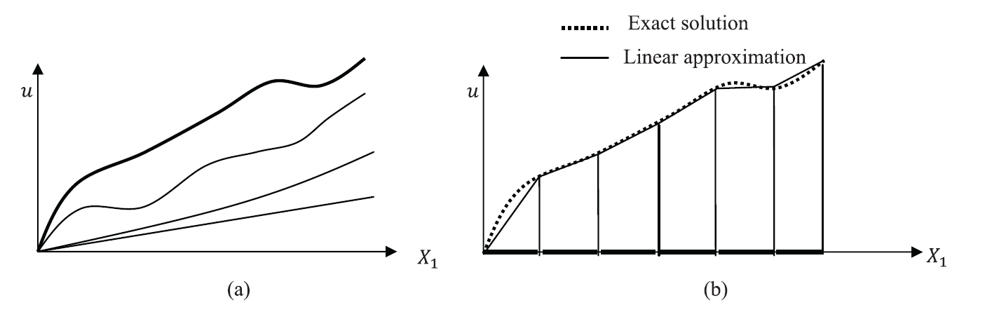
As shown in the previous chapter, the approximate methods involve assuming a particular form for the unknown variables such that the approximate solution has a finite number of unknown parameters. The approximate solution, or often termed trial function, that were used in the previous section were often polynomials which are continuous and differentiable along the whole domain (Figure 1a). The finite element analysis, however, involves using piecewise linear (piecewise affine) or piecewise nonlinear functions for the approximate solution (Figure 1b). Afterwards, a weak formulation of the problem is solved using the Virtual Work method (which as shown previously is equivalent to the Galerkin method).

Interpolation Order

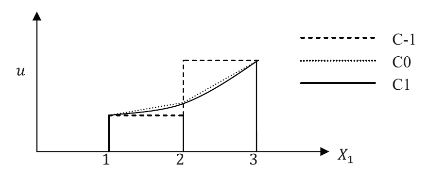
In traditional finite element analysis, the values of the displacements at specific points (nodes) across the domain are the main unknowns to be calculated using the method. The displacements at intermediate locations between the nodes are interpolated according to a chosen interpolation function. The interpolation functions are classified according to their differentiability. A interpolation function is an interpolation function that can be differentiated n times while an interpolation function that is discontinuous across nodes is termed . Figure 2 shows three nodes (node 1, node 2 and node 3) and three different interpolation functions for the displacement at intermediate locations between the nodes. Figure 2 illustrates discontinuous , continuous , and once differentiable interpolation functions.