Engineering at Alberta Courses

Plane Beam Approximations: Timoshenko Beam

The Timoshenko beam formulation is intentionally derived to better describe beams whose shear deformations cannot be ignored. Short beams are a prime example for such beams, and thus, the Timoshenko beam approximation is better suited to describe their behaviour. The basic physical assumptions behind the Timoshenko beam are similar to those described for the Euler Benroulli beam, except that shear deformations are allowed. The following are the three basic assumptions behind the Timoshenko beam theory. (Compare with those described above for the Euler Bernoulli beam)

Plane sections perpendicular to the neutral axis before deformations remain plane, but not necessarily perpendicular to the neutral axis after deformation (Figure 6).
The deformations are small.
The beam is linear elastic isotropic and Poisson’s ratio effects are ignored.

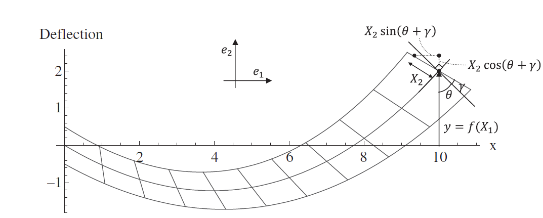
Similar to the Euler Bernoulli beam, the Timoshenko beam is assumed to lie such that its long axis is aligned with $X_1$ . The deformation is controlled by two functions: $y(X_1)$ which describes the deformation of the neutral axis (Figure 6) and $\gamma(X_1)$ which describes the shear rotation of the cross section. In essence, the total rotation of the cross section is equal to $y'(X_1)+\gamma(X_1)$ . The coordinates of an arbitrary point $p$ before deformation are given by:

$X=\left(\begin{array}{c}X_1^p\\X_2^p\\X_3^p\end{array}\right)$

Ignoring any effect due to Poisson’s ratio, the coordinates of the point $p$ after deformation (Figure 6) are given by:

$x=\left(\begin{array}{c}X_1^p-X_2^p\sin{(y'+\gamma)}\\y+X_2^p\cos{(y'+\gamma)}\\X_3^p\end{array}\right)$

Setting $\psi=y'+\gamma$ , the small deformations assumption allows the approximations $\psi\approx \sin{\psi}\approx \tan{\psi}$ and $\cos{\psi}\approx 1$ . Therefore, the displacement function after incorporating the small deformations assumption is given by:

$u=x-X=\left(\begin{array}{c}-X_2^p\psi\\y\\0\end{array}\right)$

We can drop the superscript p since this applies to any arbitrary point. We also note that $y'=\tan{\theta}\approx \theta$ . Therefore, the displacement function has the form:

$u=x-X=\left(\begin{array}{c}-X_2\psi\\y\\0\end{array}\right)$

we remind the reader that $y$ and $\gamma$ (and hence $\psi=y'+\gamma$ ) are functions of $X_1$ only. Therefore, The gradient of the displacement matrix is given by:

$\nabla u=\left(\begin{matrix}-X_2\frac{\mathrm{d}\psi}{\mathrm{d}X_1} & -\psi & 0 \\\frac{\mathrm{d}y}{\mathrm{d}X_1} & 0 & 0\\0&0&0\end{matrix}\right)$

Therefore, the small strain matrix has the form:

$\varepsilon=\frac{1}{2}\left(\nabla u + \nabla u^T\right)=\left(\begin{matrix}-X_2\frac{\mathrm{d}^\psi}{\mathrm{d}X_1} & -\frac{\gamma}{2} & 0 \\-\frac{\gamma}{2} & 0 & 0\\0&0&0\end{matrix}\right)$

In essence, the deformation assumptions result in all of the strain components being zero except for $\varepsilon_{11}$ and $\varepsilon_{12}=\varepsilon_{21}$ . Furthermore, we will look carefully at the variation of $\varepsilon_{11}$ on a given cross section. For a given cross section of the beam we have $X_1$ is equal to constant. Therefore, the quantity $\frac{\mathrm{d}\psi}{\mathrm{d}X_1}$ is constant on the cross section and therefore $\varepsilon_{11}$ is linear in the vertical direction (Figure 2). The value of $\varepsilon_{11}$ is equal to zero at the neutral axis $X_2=0$ . The positive convention for \psi and for $\psi'$ lead to a positive strain below the neutral axis with the maximum positive value $\varepsilon_a$ at the bottom fibre of the cross section. The positive convention also leads to a negative strain above the neutral axis with the maximum negative value $\varepsilon_b$ at the top fibre of the cross section. On the other hand $\varepsilon_{12}$ is constant on the cross section. Using the linear elastic constitutive relationship for the beam material and ignoring Poisson’s ratio lead to the same distribution for $\sigma_{11}=E\varepsilon_{11}$ (Figure 2). Therefore, the normal stress component distribution on the cross section is given by:

(7) $\begin{equation*}\sigma_{11}=-EX_2\frac{\mathrm{d}\psi}{\mathrm{d}X_1}=-EX_2\left(\frac{\mathrm{d}^2y}{\mathrm{d}X_1^2}+\frac{\mathrm{d}\gamma}{\mathrm{d}X_1}\right)\end{equation*}$

The internal bending moment on the cross section can be obtained using the integral:

(8) $\begin{equation*}M=\int\int\! -\sigma_{11}X_2 \,\mathrm{d}X_2\mathrm{d}X_3=\int\int\! E\frac{\mathrm{d}\psi}{\mathrm{d}X_1}X_2^2 \,\mathrm{d}X_2\mathrm{d}X_3=EI\frac{\mathrm{d}\psi}{\mathrm{d}X_1}\end{equation*}$

The shear stress distribution on the cross section is given by:

$\sigma_{12}=kG(2\varepsilon_{12})=-kG\gamma$

where $G$ is the shear modulus and $k$ is a constant introduced to allow for averaging or smearing the shear stress over the full cross section. $k$ was introduced by Timoshenko in his book. For more information on $k$ you can view this reference. The shear force is the integral of this average $\sigma_{12}$ over the cross section which yields:

$V=\int\int \! -\sigma_{12} \, \mathrm{d}X_2\mathrm{d}X_3=\int\int \! kG\gamma \, \mathrm{d}X_2\mathrm{d}X_3=kA G\gamma$

In essence, the term $kA$ gives the corresponding “effective” shear area such that the shear stress is equal to $\frac{V}{kA}$ .

Equilibrium Equations:

The equilibrium Equation 4 developed for the Eulber Bernoulli beam also applies to the Timoshenko beam (Figure 4). By substituting for $M$ using Equation 8 in the equilibrium equations, we reach:

(9) $\begin{equation*}EI\frac{\mathrm{d}^3\psi}{\mathrm{d}X_1^3}=q\end{equation*}$

We also have the following differential equation in terms of the beam displacement $y$ :

$y'=\psi-\gamma\Rightarrow y'=\frac{\mathrm{d}y}{\mathrm{d}X_1}=\psi - \frac{V}{kAG}\Rightarrow$

(10) $\begin{equation*}\frac{\mathrm{d}y}{\mathrm{d}X_1}=\psi - \frac{EI}{kAG}\frac{\mathrm{d}^2\psi}{\mathrm{d}X_1^2}\end{equation*}$

The solution for y and \psi have the following forms:

$\begin{split}EI\psi & =\int\int\int \!q \, \mathrm{d}X_1 \mathrm{d}X_1 \mathrm{d}X_1 + C_1\frac{X_1^2}{2}+C_2X_1+C_3\\EI y & =\int\int\int\int \!q \, \mathrm{d}X_1 \mathrm{d}X_1 \mathrm{d}X_1\mathrm{d}X_1+C_1\frac{X_1^3}{6}+C_2\frac{X_1^2}{2}+C_3X_1+C_4\\& -\frac{EI}{kAG}\left(\int\int \!q \, \mathrm{d}X_1 \mathrm{d}X_1+C_1X_1\right) \end{split}$

The above two equations (Equation 9 and Equation 10) can be solved if four boundary conditions for the cross section rotation $\psi$ , the moment $M=EI\frac{\mathrm{d}\psi}{\mathrm{d}X_1}$ , the shear $V=EI\frac{\mathrm{d}^2\psi}{\mathrm{d}X_1^2}$ , and/or the displacement $y$ are available. At least one boundary condition for y has to be given in order to find the integration constant $C_4$ . Note that if $kAG>>EI$ then the Timoshenko beam solution would approach the Euler Bernoulli beam solution.

Open Educational Resources

Plane Beam Approximations: Timoshenko Beam

Equilibrium Equations:

Video

Quiz – Timoshenko Beam

Leave a Reply Cancel reply