
Stress: Cauchy Sensor Tensor
Learning Outcomes
- Identify that in a continuum, stress at a point is defined using a symmetric matrix, and not a number. Describe what the components of the matrix mean.
- Identify that the stress matrix is symmetric. Recognize the implications as having a coordinate system in which no shear stresses appear in the matrix. Employ the process of diagonalization of a symmetric matrix to find this coordinate system.
- Compute the normal and shear stresses on different planes using a stress matrix.
Definitions
The topics presented here were first introduced by Augustin-Louis Cauchy in the nineteenth century. Cauchy introduced the idea of stress or traction vectors which are force vectors per unit area. He then introduced the stress as a  symmetric matrix. The stress matrix is perhaps one of the early concepts that promoted the study of vectors and matrices. The word
  that is used to describe a matrix is perhaps due to the fact, as will be shown here, that the stress tensor acts on area vectors to produce traction vectors.
Traction Vector
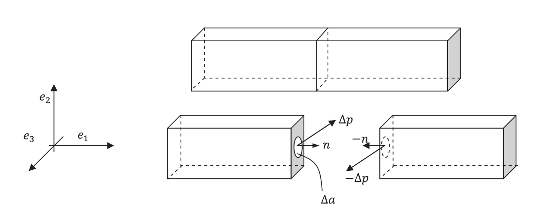
Before defining the “Stress Tensor/Matrix”, we first define the force vector per unit area. The force vector per unit area is termed the “Traction Vector”. The traction vector at a point inside a body can be defined after removing the adjacent material and considering that a force vector  is exerted by the removed material on an area
  surrounding that point. The traction vector
  at this point considering the surface with the normal vector
  is then (Figure 1 ):
![\[t_{n} = \lim_{\Delta \to 0} \frac{\Delta p}{\Delta a}\]](https://engcourses-uofa.ca/wp-content/ql-cache/quicklatex.com-1254ffe17403bf7142def4680dea15aa_l3.png "Rendered by QuickLaTeX.com")
By invoking Newton’s third law of motion (every action has an equal and opposite reaction), the traction vector acting on the corresponding point on the removed material whose normal vector is -n is equal to (Figure 1 ):
![\[t_{-n} = -t_{n}\]](https://engcourses-uofa.ca/wp-content/ql-cache/quicklatex.com-80d13d6b5a68f8f8d5d9fd4dbd73f07d_l3.png "Rendered by QuickLaTeX.com")
 acting at a point in an area with normal vector
The Cauchy Stress Tetrahedron
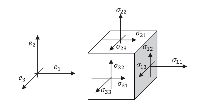
In this section we present the proof according to the French Mathematician Augustin-Louis Cauchy that shows that the state of stress at a particular point inside a continuum is well defined using a symmetric matrix, which is called the stress matrix or stress tensor. Knowing this matrix allows the calculation of any traction vector on any plane passing through that point. First, we consider an infinitesimal cube (Figure 2) at a point inside the material and we consider the three faces perpendicular to the three basis vectors  ,
,  , and
, and  . The force per unit area vector on each of these three faces has three components and therefore, in total, there are nine components. We then set
  as the stress component on the face with normal i and acting in the direction
  . Notice that in some textbooks, this definition could be reversed. A tetrahedron can be formed by considering four faces perpendicular to , , , and an arbitrary vector (Figure 3). We are going to use the stress components to find the traction vector acting on the arbitrary area whose normal vector is . If
  is the area of the surface with normal , then:
![\[nA_n = A_1e_1 + A_2e_2 + A_3e_3\]](https://engcourses-uofa.ca/wp-content/ql-cache/quicklatex.com-40ae6e754ea9db7c3226e56994ae0908_l3.png "Rendered by QuickLaTeX.com")
where  ,
,  , and
, and  are the areas of the triangular faces perpendicular to , , and respectively (Can you derive the above formula using the properties of the cross product?). Setting
  with
with  :
:
![\[n = n_1e_1 + n_2e_2 + n_3e_3\]](https://engcourses-uofa.ca/wp-content/ql-cache/quicklatex.com-ee006933d4cdd70a9dd6a273784782fa_l3.png "Rendered by QuickLaTeX.com")
Invoking Newton’s equations of equilibrium, the sum of the forces acting on the tetrahedron (including the gravity force  where
where  ,
,  , and
, and  are the components of the gravity acceleration) are equal to its mass multiplied by its acceleration vector
  . Therefore:
![\[-\sigma_{11}A_1 -\sigma_{21}A_2 -\sigma_{31}A_3 + t_{n1}A_n + mg_1 = ma_1\]](https://engcourses-uofa.ca/wp-content/ql-cache/quicklatex.com-d86ce87c40467bebd4ed6b4542975ba6_l3.png "Rendered by QuickLaTeX.com")
![\[-\sigma_{12}A_1 -\sigma_{22}A_2 -\sigma_{32}A_3 + t_{n2}A_n + mg_2 = ma_2\]](https://engcourses-uofa.ca/wp-content/ql-cache/quicklatex.com-57f6bc53bff76dc5b29a7c3834bb99c5_l3.png "Rendered by QuickLaTeX.com")
![\[-\sigma_{13}A_1 -\sigma_{23}A_2 -\sigma_{33}A_3 + t_{n3}A_n + mg_3 = ma_3\]](https://engcourses-uofa.ca/wp-content/ql-cache/quicklatex.com-f953de8c2bb31210ce213baa317dec7e_l3.png "Rendered by QuickLaTeX.com")
The mass  can be related to the height
  of the tetrahedron perpendicular to using the mass density
  as follows:
![\[m = \frac{\rho h A_n}{3}\]](https://engcourses-uofa.ca/wp-content/ql-cache/quicklatex.com-120f2eae8bb5e621f94e752f8c710781_l3.png "Rendered by QuickLaTeX.com")
Substituting for in the equilibrium equations, rearranging, and taking the limit as the volume of the tetrahedron goes to zero, (i.e., as  ) lead to the linear relationship between the traction vector and the unit normal vector :
![\[\begin{pmatrix} t_{n1} \\ t_{n2} \\ t_{n3} \\ \end{pmatrix} = \begin{pmatrix} \sigma_{11} & \sigma_{21} & \sigma_{31} \\ \sigma_{12} & \sigma_{22} & \sigma_{32} \\ \sigma_{13} & \sigma_{23} & \sigma_{33} \\ \end{pmatrix} \begin{pmatrix} n_1 \\ n_2 \\ n_3 \\ \end{pmatrix}\]](https://engcourses-uofa.ca/wp-content/ql-cache/quicklatex.com-f87ee73a892b05e448918c647bd9fcfc_l3.png "Rendered by QuickLaTeX.com")
Therefore:
![\[t_n = \sigma^Tn\]](https://engcourses-uofa.ca/wp-content/ql-cache/quicklatex.com-e95d15b6ce9ac7ccd6c86842cc9655b1_l3.png "Rendered by QuickLaTeX.com")
I.e., the Cauchy stress tensor  is a linear operator that acts as a linear function from
  such that
  where is a unit vector, the result
  is the traction vector (force vector per unit area) acting on the surface with normal .
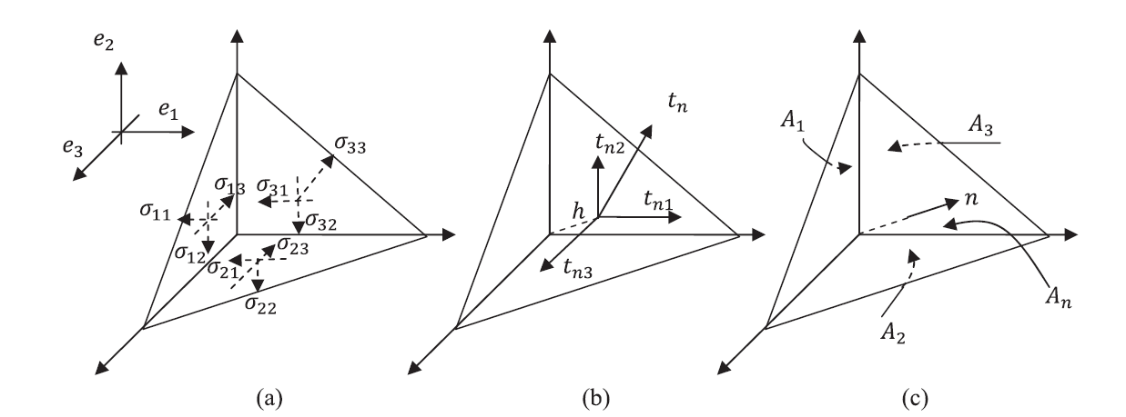 on the inclined face. (c) Areas of the different faces.
Symmetry of the Stress Matrix
Because of moment equilibrium whether the body is in static or dynamic equilibrium, it will be shown that in common materials, the Cauchy Stress Tensor is a symmetric tensor, i.e.,  . According to Euler’s laws of motion, the rate of change of the angular momentum
  in the material is equal to the moment of the external forces. Euler’s laws can be applied to an
infinitesimal cuboid with external forces acting on its faces as shown in Figure 4. The moment around the axis perpendicular to the plane shown and passing through the bottom left corner (black dot), neglecting smaller quantities, can be evaluated as follows:
in the material is equal to the moment of the external forces. Euler’s laws can be applied to an
infinitesimal cuboid with external forces acting on its faces as shown in Figure 4. The moment around the axis perpendicular to the plane shown and passing through the bottom left corner (black dot), neglecting smaller quantities, can be evaluated as follows:
![\[M_{external} = (\sigma_{12} - \sigma_{21})\Delta x_1 \Delta x_2 \Delta x_3\]](https://engcourses-uofa.ca/wp-content/ql-cache/quicklatex.com-ddbd2c22c7a116d99d0af9248a7b4ced_l3.png "Rendered by QuickLaTeX.com")
Assuming the cuboid rotates around the bottom left corner with angular velocity  , then
  has the following form:
![\[\dot{L} = \rho\dot{\omega} I = \rho\dot{\omega} (\frac{1}{3} \Delta x_1 \Delta x_2 \Delta x_3 (\Delta x_2^2 + \Delta x_1^2))\]](https://engcourses-uofa.ca/wp-content/ql-cache/quicklatex.com-682e7479430c704bcaa0e223ca20b6eb_l3.png "Rendered by QuickLaTeX.com")
where is the density,  is the angular acceleration and I is the polar moment of inertia. Equating
  with and taking the limit as the volume goes to zero(
 ,
, ):
):
![\[\sigma_{12} = \sigma_{21}\]](https://engcourses-uofa.ca/wp-content/ql-cache/quicklatex.com-55e79748c1b56cb7ef5b71649b2bff85_l3.png "Rendered by QuickLaTeX.com")
Similarly,  and
and  . Therefore:
![\[\sigma = \sigma^T\]](https://engcourses-uofa.ca/wp-content/ql-cache/quicklatex.com-0e318dad9bab79f6c48be7b5baa34a22_l3.png "Rendered by QuickLaTeX.com")
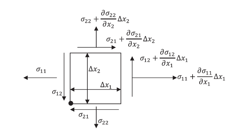 of an infinitesimal cuboid with dimensions ,
  , and
, and  .
.Normal and Shear Stress
Given a state of stress described by and given a plane with perpendicular , the normal stress  is a real number representing the component of the force acting perpendicular to that plane and is given by (positive for tension and negative for compression):
![\[(1) \sigma_n = t_n \cdot n\]](https://engcourses-uofa.ca/wp-content/ql-cache/quicklatex.com-c51feb5a39adec11e1fdbb92182c2fd3_l3.png "Rendered by QuickLaTeX.com")
While the shear stress  is the magnitude of the component of the traction vector acting parallel to the surface of the plane:
![\[\tau_n = \|t_n - \sigma_nn\|\]](https://engcourses-uofa.ca/wp-content/ql-cache/quicklatex.com-11c9ee6ac70d56a5fe111479887f754a_l3.png "Rendered by QuickLaTeX.com")
Two Dimensional Illustrative Example
In this example a two dimensional state of stress at a point is described by the Cauchy stress tensor  . Consider a plane with normal . The black arrow in the figure below indicates the direction of the plane, the traction vector is indicated by the blue arrow, the green arrow (outwards indicate tension and inwards indicate compression) shows the normal stress while the red arrow indicates the direction of the shear stress vector. The values are given next to the table. Try it out by changing the values in the boxes below and hitting enter (Notice that the vector n is normalized before any computations are performed):
Try to answer the following questions:
Find a state of stress and a direction when the green arrow is pointing opposite to the black arrow. What happens to the directions of the other vectors?
Find a state of stress and a direction such that the normal stress is zero while the shear stress is not and vice versa. What happens to the stress state when you change
in each case? What happens when you choose n to be horizontal or vertical?
What happens when you choose values for the stress components such that
 and
and  ?
?
Three Dimensional Illustrative Example
Now try to answer the same questions on the three dimensional example below by changing the values in the box and hitting enter:
Principal Stresses and Principal Directions
Since is symmetric, there exists a coordinate system in which the component form of is diagonal, i.e., there is a coordinate transformation such that the planes perpendicular to the coordinate system have no shear stresses! This coordinate system is the one aligned with the eigenvectors of the stress tensor. The eigenvectors are called “The Principal Directions” while the eigenvalues are called “The Principal Stresses”.
The principal stresses are denoted  ,
,  and
and  . If
. If  ,
,  and
and  are the corresponding normalized eigenvectors, then
![\[Q = \begin{pmatrix} ev_{11} & ev_{12} & ev_{13} \\ ev_{21} & ev_{22} & ev_{23} \\ ev_{31} & ev_{32} & ev_{33} \\ \end{pmatrix}\]](https://engcourses-uofa.ca/wp-content/ql-cache/quicklatex.com-b681f4ab22c32eb6386ab3226450ca8d_l3.png "Rendered by QuickLaTeX.com")
is an orthogonal matrix of transformation into the coordinate system described by the eigenvectors. The order of the eigenvectors should be chosen to preserve the right hand orientation of the new coordinate system and in this case  is a rotation. The stress matrix in this particular coordinate system will be diagonal:
![\[\sigma ' = Q\sigma Q^T = \begin{pmatrix} \sigma_1 & 0 & 0 \\ 0 & \sigma_2 & 0 \\ 0 & 0 & \sigma_3 \\ \end{pmatrix}\]](https://engcourses-uofa.ca/wp-content/ql-cache/quicklatex.com-135232b87a5dbbbc5476371e7e870046_l3.png "Rendered by QuickLaTeX.com")
Two Dimensional Illustrative Example
Consider a two dimensional state of stress at a point described by the Cauchy stress tensor . The square on the left in the figure below is aligned with the original coordinate system. The red and blue arrows represent the traction vectors acting on the horizontal and vertical planes, respectively. The example below finds the eigenvalues and eigenvectors of the stress matrix. Then, a coordinate transformation described by the matrix whose rows represent the eigenvectors of is used to rotate everything into that new coordinate system. In the new coordinate system, the force vectors are perpendicular to the faces of the square!
Three Dimensional Illustrative Example
Similarly, the example below illustrates the concept of rotating a cube into the coordinate system described by the eigenvectors of . The sizes of the arrows showing the traction or principal stress vectors qualitatively represent the magnitudes of the vectors. I.e they are not proportionate to the magnitude but only represent which vector has the larger or smaller magnitude relative to others.
Mohr’s Circle for Plane Stress
Visit Wikipedia’s entry on Mohr Circle to learn about the history, the construction and the applications of Mohr’s circle!
In the following example, you can change the values of the stress matrix entries from -10 to 10 units to reconstruct Mohr’s circle. The black arrow indicates the point on the circle corresponding to a plane oriented at an angle (theta) with respect to the dotted line which corresponds to the plane perpendicular to the horizontal direction. The angle on the circle between the dotted and solid arrows is (2theta).
thanks for this useful paper it is the best in this subject
Thanks for the best subject … this is very usefull .. I have some query about three D coordinate transformation
Dear University of Alberta
What a great page. This is a very important topic and this page makes it look simple.
Thank you so much for caring for the students who need this!!!!!