Engineering at Alberta Courses » Euler Bernoulli Beams under Lateral Loading

Approximate Methods: The Rayleigh Ritz Method: Euler Bernoulli Beams under Lateral Loading

Learning Outcomes

Describe the steps required to find an approximate solution for a beam system (and the extension to a continuum) using the Rayleigh Ritz method. (Step1: Assume a displacement function, apply the BC. Step 2: Write the expression for the PE of the system. Step 3: Find the minimizers of the PE of the system.)
Employ the RR method to compute an approximate solution for the displacement in an Euler Bernoulli beam(and the extension to a continuum).
Differentiate between the requirement for an approximate solution and an exact solution.

Euler Bernoulli Beams under Lateral Loading

For plane Euler Bernoulli beams under lateral loading, the unknown displacement function is $y$ . In this case, the potential energy of the system has the following form (See Euler Bernoulli Beam and energy expressions):

$PE=\mbox{Total Strain Energy} - W=\int\!\frac{EI}{2}\left(\frac{\mathrm{d}^2y}{\mathrm{d}X_1^2}\right)^2 \,\mathrm{d}X_1 - W$

where $E$ is Young’s modulus, $I$ is the moment of inertia, and $W$ is the work done by all the external forces acting on the bar (concentrated forces and distributed loads). A few examples to solve for the displacements, rotations, shear forces, and moments for an Euler Bernoulli beam under lateral loading are presented in this section. Similar to the previous section, the Rayleigh Ritz method starts by choosing a form for the displacement function. This form has to satisfy the “essential” boundary conditions, which for this particular type of problems are those boundary conditions imposed on the displacements and the rotations. The following examples show the method for different external loads, and beam configurations.

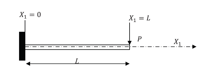
Example 1: Cantilever Beam

Let a beam with a length $L$ and a constant cross sectional parameters area $A$ and moment of inertia $I$ be aligned with the coordinate axis $X_1$ . Assume that the beam is subjected to a constant force of value $P$ applied at the end $X_1=L$ in the direction shown in the figure. Assume that the bar is fixed (rotation and displacement are equal to zero) at the end $X_1=0$ . Find the displacement, rotation, bending moment, and shearing forces on the beam by directly solving the differential equation of equilibrium and then using the Rayleigh Ritz method assuming polynomials of the degrees (0,1, 2, 3, and 4). Assume the beam to be linear elastic with Young’s modulus $E$ and that the Euler Bernoulli Beam is an appropriate beam approximation.

Solution

Exact Solution:
First, the exact solution that would satisfy the equilibrium equations can be obtained. The equilibrium equation as shown in the Euler Bernoulli beam section when $E$ and $I$ are constant is:

$EI\frac{\mathrm{d}^4y}{\mathrm{d}X_1^4}=q$

For the shown cantilever beam, $q=0$ and therefore the exact solution for the displacement $y$ has the form:

$y=\frac{C_1X_1^3}{6}+\frac{C_2X_1^2}{2}+C_3X_1+C_4$

where the constants can be obtained from the boundary conditions:

$\begin{split} & @X_1=0:y=0\Rightarrow C_4=0\\ & @X_1=0:\theta=\frac{\mathrm{d}y}{\mathrm{d}X_1}=0\Rightarrow C_3=0\\ & @X_1=L:M=0\Rightarrow EI\frac{\mathrm{d}^2y}{\mathrm{d}X_1^2}=0\Rightarrow C_2=-C_1L\\ & @X_1=L:V=P\Rightarrow EI\frac{\mathrm{d}^3y}{\mathrm{d}X_1^3}=P\Rightarrow C_1=\frac{P}{EI} \end{split}$

Therefore, the exact solution for the displacement $y$ , the rotation $\theta$ , the moment $M$ , and the shear $V$ are:

$\begin{split} y & =\frac{PX_1^3}{6EI}-\frac{PLX_1^2}{2EI}\\ \theta & = \frac{\mathrm{d}y}{\mathrm{d}X_1}=\frac{PX_1^2}{2EI}-\frac{PLX_1}{EI}\\ M & = EI\frac{\mathrm{d}^2y}{\mathrm{d}X_1^2}=PX_1-PL\\ V & = EI\frac{\mathrm{d}^3y}{\mathrm{d}X_1^3}=P \end{split}$

The Rayleigh Ritz Method:
The first step in the Rayleigh Ritz method finds the minimizer of the potential energy of the system which can be written as:

$PE=\int\!\overline{U}\,dX - W=\int_0^L\!\frac{EI}{2}\left(\frac{\mathrm{d}^2y}{\mathrm{d}X_1^2}\right)^2 \,\mathrm{d}X_1 - (-P)y|_{X_1=L}$

Notice that the potential energy lost by the action of the end force $P$ is equal to the product of – $P$ ( $P$ is acting downwards and $y$ is assumed upwards) and the displacement $y$ evaluated at $X_1= L$ . To find an approximate solution, an assumption for the shape or the form of $y$ has to be introduced.
Polynomials of the Zero and First Degrees:
If we assume that $y$ is a constant (polynomial of the zero degree) or a linear (polynomial of the first degree) function, and when attempting to satisfy the essential boundary conditions:

$\begin{split} @X_1=0 & :y=0\\ @X_1=0 & :\theta=\frac{\mathrm{d}y}{\mathrm{d}X_1}=0 \end{split}$

this leads to the trivial solution $y= 0$ , which will automatically be rejected.

Polynomial of the Second Degree:
The approximate solution forms for the displacement $y$ , the rotation $\theta$ , the moment $M$ , and the shear force $V$ functions if $y$ is assumed to be a polynomial of the second degree are:

$\begin{split} y & =a_2X_1^2+a_1X_1+a_0\\ \theta &=\frac{\mathrm{d}y}{\mathrm{d}X_1} =2a_2X_1+a_1\\ M &=EI\frac{\mathrm{d}^2y}{\mathrm{d}X_1^2} =2EIa_2\\ V &=0 \end{split}$

To satisfy the essential boundary conditions, we have:

$\begin{split} @X_1=0 & :y=0\Rightarrow a_0=0\\ @X_1=0 & :\theta=\frac{\mathrm{d}y}{\mathrm{d}X_1}=0\Rightarrow a_1=0 \end{split}$

Therefore, the solutions forms have only one parameter $a_2$ that can be controlled:

$\begin{split} y & =a_2X_1^2\\ \theta &=\frac{\mathrm{d}y}{\mathrm{d}X_1} =2a_2X_1\\ M &=EI\frac{\mathrm{d}^2y}{\mathrm{d}X_1^2} =2EIa_2\\ V &=0 \end{split}$

Substituting into the equation of the potential energy of an Euler Bernoulli beam:

$PE=\frac{EI}{2}\int_0^L\!\left(2a_2\right)^2\,\mathrm{d}X_1+P\left(a_2L^2\right)$

The unknown coefficient $a_2$ can be obtained by minimizing the potential energy:

$\frac{\mathrm{d} PE}{\mathrm{d} a_2} =4EILa_2+PL^2=0\Rightarrow a_2=-\frac{PL}{4EI}$

Therefore, the “best” parabolic approximation for $y$ along with the corresponding solutions for $\theta, M$ , and $V$ are given by:

$\begin{split} y & =-\frac{PLX_1^2}{4EI}\\ \theta &=\frac{\mathrm{d}y}{\mathrm{d}X_1} =-\frac{PLX_1}{2EI}\\ M &=EI\frac{\mathrm{d}^2y}{\mathrm{d}X_1^2} =-\frac{PL}{2}\\ V &=EI\frac{\mathrm{d}^3y}{\mathrm{d}X_1^3} =0 \end{split}$

Note that because of the simplicity of the approximation, the shear force (which is the third derivative) is always equal to zero.

Polynomial of the Third Degree:
The approximate solution forms for the displacement $y$ , the rotation $\theta$ , the moment $M$ , and the shear force $V$ functions if $y$ is assumed to be a polynomial of the third degree are:

$\begin{split} y & =a_3X_1^3+a_2X_1^2+a_1X_1+a_0\\ \theta &=\frac{\mathrm{d}y}{\mathrm{d}X_1} =3a_3X_1^2+2a_2X_1+a_1\\ M &=EI\frac{\mathrm{d}^2y}{\mathrm{d}X_1^2} =6EIa_3X_1+2EIa_2\\ V &=6EIa_3 \end{split}$

To satisfy the essential boundary conditions, we have:

$\begin{split} @X_1=0 & :y=0\Rightarrow a_0=0\\ @X_1=0 & :\theta=\frac{\mathrm{d}y}{\mathrm{d}X_1}=0\Rightarrow a_1=0 \end{split}$

Therefore, the solutions forms have only two parameters $a_2$ and $a_3$ that can be controlled:

$\begin{split} y & =a_3X_1^3+a_2X_1^2\\ \theta &=\frac{\mathrm{d}y}{\mathrm{d}X_1} =3a_3X_1^2+2a_2X_1\\ M &=EI\frac{\mathrm{d}^2y}{\mathrm{d}X_1^2} =6EIa_3X_1+2EIa_2\\ V &=6EIa_3 \end{split}$

Substituting into the equation of the potential energy of an Euler Bernoulli beam:

$PE=\frac{EI}{2}\int_0^L\!\left(6a_3X_1+2a_2\right)^2\,\mathrm{d}X_1+P\left(a_3L^3+a_2L^2\right)$

The unknown coefficients $a_2$ and $a_3$ can be obtained by minimizing the potential energy:

$\begin{split} \frac{\partial PE}{\partial a_2} & =\frac{EI}{2}(8a_2L+12a_3L^2)+PL^2=0\\ \frac{\partial PE}{\partial a_3} & =\frac{EI}{2}(12a_2L^2+24a_3L^3)+PL^3=0 \end{split}$

Solving the above two equations yields:

$a_2=-\frac{PL}{2EI} \qquad a_3=\frac{P}{6EI}$

Therefore, the “best” cubic approximation for $y$ along with the corresponding solutions for $\theta, M$ , and $V$ are given by:

$\begin{split} y & =\frac{PX_1^3}{6EI}-\frac{PLX_1^2}{2EI}\\ \theta &=\frac{\mathrm{d}y}{\mathrm{d}X_1} =\frac{PX_1^2}{2EI}-\frac{PLX_1}{EI}\\ M &=EI\frac{\mathrm{d}^2y}{\mathrm{d}X_1^2} =PX_1-PL\\ V &=EI\frac{\mathrm{d}^3y}{\mathrm{d}X_1^3} =P \end{split}$

The “approximate” solution obtained here is identical to the “exact” solution obtained above. This is because the trial function for $y$ was assumed to be a cubic polynomial and the exact solution is in fact a cubic polynomial. One should note that when the “form” or “shape” of the approximate solution contains the “form” or “shape” of the exact solution, then the Rayleigh Ritz method renders the exact solution! To see this, we are going to try a finer approximation (A polynomial of the fourth degree).

Polynomial of the Fourth Degree:
The approximate solution forms for the displacement $y$ , the rotation $\theta$ , the moment $M$ , and the shear force $V$ functions if $y$ is assumed to be a polynomial of the fourth degree are:

$\begin{split} y & =a_4X_1^4+a_3X_1^3+a_2X_1^2+a_1X_1+a_0\\ \theta &=\frac{\mathrm{d}y}{\mathrm{d}X_1} =4a_4X_1^3+3a_3X_1^2+2a_2X_1+a_1\\ M &=EI\frac{\mathrm{d}^2y}{\mathrm{d}X_1^2} =12EIa_4X_1^2+6EIa_3X_1+2EIa_2\\ V &=24EIa_4X_1+6EIa_3 \end{split}$

To satisfy the essential boundary conditions, we have:

$\begin{split} @X_1=0 & :y=0\Rightarrow a_0=0\\ @X_1=0 & :\theta=\frac{\mathrm{d}y}{\mathrm{d}X_1}=0\Rightarrow a_1=0 \end{split}$

Therefore, the solutions forms have the parameters $a_2, a_3$ , and $a_4$ that can be controlled:

$\begin{split} y & =a_4X_1^4+a_3X_1^3+a_2X_1^2\\ \theta &=\frac{\mathrm{d}y}{\mathrm{d}X_1} =4a_4X_1^3+3a_3X_1^2+2a_2X_1\\ M &=EI\frac{\mathrm{d}^2y}{\mathrm{d}X_1^2} =12EIa_4X_1^2+6EIa_3X_1+2EIa_2\\ V &=24EIa_4X_1+6EIa_3 \end{split}$

Substituting into the equation of the potential energy of an Euler Bernoulli beam:

$PE=\frac{EI}{2}\int_0^L\!\left(12a_4X_1^2+6a_3X_1+2a_2\right)^2\,\mathrm{d}X_1+P\left(a_4L^4+a_3L^3+a_2L^2\right)$

The unknown coefficients $a_2, a_3$ , and $a_4$ can be obtained by minimizing the potential energy:

$\frac{\partial PE}{\partial a_2} =0\qquad \frac{\partial PE}{\partial a_3} =0 \qquad \frac{\partial PE}{\partial a_4} =0$

Solving the above three equations yields:

$a_2=-\frac{PL}{2EI} \qquad a_3=\frac{P}{6EI} \qquad a_4=0$

Therefore, assuming a fourth order polynomial gives the same solution as a third order polynomial!

View Mathematica Code

(*Exact Solution*)Clear[a, x, V, M, P, y, L, EI]
M = EI*D[y[x], {x, 2}];
V = EI*D[y[x], {x, 3}];
th = D[y[x], x];
q = 0;
M1 = M /. x -> 0;
M2 = M /. x -> L;
V1 = V /. x -> 0;
V2 = V /. x -> L;
y1 = y[x] /. x -> 0;
y2 = y[x] /. x -> L;
th1 = th /. x -> 0;
th2 = th /. x -> L;
s = DSolve[{EI*y''''[x] == q, y1 == 0, th1 == 0, V2 == P, M2 == 0}, y,
    x];
y = y[x] /. s[[1]]
th = D[y, x]
M = EI*D[y, {x, 2}]
V = EI*D[y, {x, 3}]
(*Second Degree*)
Clear[y, x, M, V, th, EI, PE]
y = a2*x^2
th = D[y, x];
M = EI*D[y, {x, 2}];
V = EI*D[y, {x, 3}];
PE = EI/2*Integrate[D[y, {x, 2}]^2, {x, 0, L}] + P*(y /. x -> L);
Eq2 = D[PE, a2];
Sol = Solve[{Eq2 == 0}, {a2}]
y = y /. Sol[[1]]
th /. Sol[[1]]
FullSimplify[M /. Sol[[1]]]
FullSimplify[V /. Sol[[1]]]
(*Third Degree*)
Clear[y, x, M, V, th, EI, PE]
y = a3*x^3 + a2*x^2
th = D[y, x];
M = EI*D[y, {x, 2}];
V = EI*D[y, {x, 3}];
PE = EI/2*Integrate[D[y, {x, 2}]^2, {x, 0, L}] + P*(y /. x -> L);
Eq1 = D[PE, a3];
Eq2 = D[PE, a2];
Sol = Solve[{Eq1 == 0, Eq2 == 0}, {a3, a2}]
y = y /. Sol[[1]]
th /. Sol[[1]]
FullSimplify[M /. Sol[[1]]]
FullSimplify[V /. Sol[[1]]]
(*Fourth Degree*)
Clear[y, x, M, V, th, EI, PE]
y = a4*x^4 + a3*x^3 + a2*x^2
th = D[y, x];
M = EI*D[y, {x, 2}];
V = EI*D[y, {x, 3}];
PE = EI/2*Integrate[D[y, {x, 2}]^2, {x, 0, L}] + P*(y /. x -> L);
Eq1 = D[PE, a3];
Eq2 = D[PE, a2];
Eq3 = D[PE, a4];
Sol = Solve[{Eq1 == 0, Eq2 == 0, Eq3 == 0}, {a3, a2, a4}]
y = y /. Sol[[1]]
th /. Sol[[1]]
FullSimplify[M /. Sol[[1]]]
FullSimplify[V /. Sol[[1]]]

View Python Code

from sympy import *
import sympy as sp 
sp.init_printing(use_latex = "mathjax")
x, EI, P, q, a2, a3, a4 = symbols("x EI P q a_2 a_3 a_4")
display("Exact")
y = Function("y")
th = y(x).diff(x)
M = EI*y(x).diff(x,2)
V = EI*y(x).diff(x,3)
q = 0
M1 = M.subs(x,0)
M2 = M.subs(x,L)
V1 = V.subs(x,0)
V2 = V.subs(x,L)
y1 = y(x).subs(x,0)
y2 = y(x).subs(x,L)
th1 = th.subs(x,0)
th2 = th.subs(x,L)
s = dsolve(EI*y(x).diff(x,4) - q, y(x), ics = {y1:0, th1:0, V2/EI:P/EI, M2/EI:0})
y = s.rhs
th = y.diff(x)
M = EI * y.diff(x,2)
V = EI * y.diff(x,3)
display("y,th,M,V: ", y,th,M,V)
display("Second Degree")
y2 = a2*x**2
PE2 = (EI/2)*integrate(y2.diff(x,2)**2, (x,0,L))+P*y2.subs(x,L)
display("Potential Energy: ", PE2)
Eq2 = PE2.diff(a2)
Sol = solve(Eq2, a2)
display("a2", Sol)
y2 = y2.subs(a2,Sol[0])
th = y2.diff(x)
M = EI * y2.diff(x,2)
V = EI * y2.diff(x,3)
display("y,th,M,V: ", y2,th,M,V)
display("Third Degree")
y3 = a3*x**3+a2*x**2
PE3 = (EI/2)*integrate(y3.diff(x,2)**2, (x,0,L))+P*y3.subs(x,L)
display("Potential Energy: ", PE3)
Eq1_3 = PE3.diff(a3)
Eq2_3 = PE3.diff(a2)
Sol = solve((Eq1_3, Eq2_3), (a2,a3))
display("a2,a3:", Sol)
y3 = y3.subs({a2:Sol[a2], a3:Sol[a3]})
th = y3.diff(x)
M = EI * y3.diff(x,2)
V = EI * y3.diff(x,3)
display("y,th,M,V: ", y3,th,M,V)
display("Fourth Degree")
y4 = a4*x**4+a3*x**3+a2*x**2
PE4 = (EI/2)*integrate(y4.diff(x,2)**2, (x,0,L))+P*y4.subs(x,L)
display("Potential Energy: ", PE4)
Eq1_4 = PE4.diff(a3)
Eq2_4 = PE4.diff(a2)
Eq3_4 = PE4.diff(a4)
Sol = solve((Eq1_4, Eq2_4, Eq3_4), (a2,a3,a4))
display("a2,a3, a4:", Sol)
y4 = y4.subs({a2:Sol[a2], a3:Sol[a3], a4:Sol[a4]})
th = y4.diff(x)
M = EI * y4.diff(x,2)
V = EI * y4.diff(x,3)
display("y,th,M,V: ", y3,th,M,V)

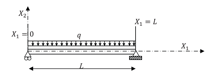
Example 2: Simple Beam

Let a beam with a length $L=10m$ and a constant moment of inertia $I=4\times 10^8 mm^4$ be aligned with the coordinate axis $X_1$ . Assume that the beam is subjected to a distributed load $q=-25kN/m$ .(Notice that the negative sign was added since $q$ is positive when it is in the direction of positive $X_2$ ). Assume that the beam is hinged at the ends $X_1= 0$ and $X_1=L$ . Find the displacement, rotation, bending moment, and shearing forces on the beam by directly solving the differential equation of equilibrium and then using the Rayleigh Ritz method assuming polynomials of the degrees (0, 1, 2, 3 and 4). Assume the beam to be linear elastic with Young’s modulus $E= 200 GPa$ and that the Euler Bernoulli Beam is an appropriate beam approximation. Compare the Rayleigh Ritz method with the exact solution.

Solution

$EI\frac{\mathrm{d}^4y}{\mathrm{d}X_1^4}=q$

For the shown simple beam, $q=-25 kN/m$ and therefore the exact solution for the displacement $y$ has the form:

$y=q\frac{X_1^4}{24}+\frac{C_1X_1^3}{6}+\frac{C_2X_1^2}{2}+C_3X_1+C_4$

where the constants can be obtained from the boundary conditions:

$\begin{split} & @X_1=0:y=0\Rightarrow C_4=0\\ & @X_1=0:M=EI\frac{\mathrm{d}^2y}{\mathrm{d}X_1^2}=0\Rightarrow C_2=0\\ & @X_1=L:y=0\Rightarrow q\frac{L^4}{24}+\frac{C_1L^3}{6}+C_3L=0\\ & @X_1=L:M=EI\frac{\mathrm{d}^2y}{\mathrm{d}X_1^2}=0\Rightarrow q\frac{L^2}{2}+C_1L=0\\ \end{split}$

therefore,

$C_1=-\frac{qL}{2}\qquad C_3=\frac{qL^3}{24}$

Therefore, the exact solution for the displacement $y$ , the rotation $\theta$ , the moment $M$ , and the shear $V$ are:

$\begin{split} y & =\frac{qX_1^4}{24EI}-\frac{qLX_1^3}{12EI}+\frac{qL^3X_1}{24EI}\\ \theta & = \frac{\mathrm{d}y}{\mathrm{d}X_1}=\frac{qX_1^3}{6EI}-\frac{qLX_1^2}{4EI}+\frac{qL^3}{24EI}\\ M & = EI\frac{\mathrm{d}^2y}{\mathrm{d}X_1^2}=\frac{qX_1^2}{2}-\frac{qLX_1}{2}\\ V & = EI\frac{\mathrm{d}^3y}{\mathrm{d}X_1^3}=qX_1-\frac{qL}{2} \end{split}$

The Rayleigh Ritz Method:
The first step in the Rayleigh Ritz method finds the minimizer of the potential energy of the system which can be written as:

$PE=\int\!\overline{U}\,dX - W=\int_0^L\!\frac{EI}{2}\left(\frac{\mathrm{d}^2y}{\mathrm{d}X_1^2}\right)^2 \,\mathrm{d}X_1 - \int_0^L \! qy\,\mathrm{d}X_1$

To find an approximate solution, an assumption for the shape or the form of $y$ has to be introduced.
Polynomials of the Zero and First Degrees:
If we assume that $y$ is a constant (polynomial of the zero degree) or a linear (polynomial of the first degree) function, and when attempting to satisfy the essential boundary conditions:

$\begin{split} @X_1=0 & :y=0\\ @X_1=L & :y=0 \end{split}$

this leads to the trivial solution $y= 0$ , which will automatically be rejected.

Polynomial of Higher Degrees:
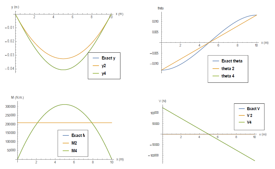
Similar to the previous examples, the coefficients are obtained by first satisfying the essential boundary conditions. Then, the remaining coefficients are obtained by minimizing the potential energy of the system. As shown in the plots below, the second and third degree trial functions give the same result, while the fourth and fifth degree trial functions give the same result. The solution is shown to give the accurate result when a polynomial of the fourth or higher degree is used.

View Mathematica Code

(*Exact Solution*)
Clear[q,EI,y,x,c1,c2,c3,c4,L]
y=(q*x^4/24+c1*x^3/6+c2*x^2/2+c3*x+c4)/EI;
Eq1=y/.x-> 0;
Eq2=y/.x-> L;
Eq3=EI*D[y,{x,2}]/.x-> 0;
Eq4=EI*D[y,{x,2}]/.x-> L;
a=Solve[{Eq1==0,Eq2==0,Eq3==0,Eq4==0},{c1,c2,c3,c4}];
y=y/.a[[1]];
theta=D[y,x]/.a[[1]];
M=FullSimplify[EI*D[y,{x,2}]/.a[[1]]];
V=FullSimplify[EI*D[y,{x,3}]/.a[[1]]];
(*Second Degree*)
y2=a2*x^2+a1*x+a0;
s=Solve[{(y2/.x-> 0)==0,(y2/.x->L)==0},{a0,a1}];
y2=y2/.s[[1]];
theta2=D[y2,x];
M2=EI*D[y2,{x,2}];
V2=EI*D[y2,{x,3}];
PE=EI/2*Integrate[(D[y2,{x,2}])^2,{x,0,L}]-Integrate[q*y2,{x,0,L}];
Eq1=D[PE,a2];
a=Solve[{Eq1==0},{a2}];
y2=y2/.a[[1]];
theta2=D[y2,x]/.a[[1]];
M2=FullSimplify[EI*D[y2,{x,2}]/.a[[1]]];
V2=FullSimplify[EI*D[y2,{x,3}]/.a[[1]]];
(*Third Degree*)
y3=a3*x^3+a2*x^2+a1*x+a0;
s=Solve[{(y3/.x-> 0)==0,(y3/.x->L)==0},{a0,a1}];
y3=y3/.s[[1]];
theta3=D[y3,x];
M3=EI*D[y3,{x,2}];
V3=EI*D[y3,{x,3}];
PE=EI/2*Integrate[(D[y3,{x,2}])^2,{x,0,L}]-Integrate[q*y3,{x,0,L}];
Eq1=D[PE,a2];
Eq2=D[PE,a3];
a=Solve[{Eq1==0,Eq2==0},{a2,a3}];
y3=y3/.a[[1]];
theta3=D[y3,x]/.a[[1]];
M3=FullSimplify[EI*D[y3,{x,2}]/.a[[1]]];
V3=FullSimplify[EI*D[y3,{x,3}]/.a[[1]]];
(*fourth Degree*)
y4=a4*x^4+a3*x^3+a2*x^2+a1*x+a0;
s=Solve[{(y4/.x-> 0)==0,(y4/.x->L)==0},{a0,a1}];
y4=y4/.s[[1]];
theta4=D[y4,x];
M4=EI*D[y4,{x,2}];
V4=EI*D[y4,{x,3}];
PE=EI/2*Integrate[(D[y4,{x,2}])^2,{x,0,L}]-Integrate[q*y4,{x,0,L}];
Eq1=D[PE,a2];
Eq2=D[PE,a3];
Eq3=D[PE,a4];
a=Solve[{Eq1==0,Eq2==0,Eq3==0},{a2,a3,a4}];
y4=y4/.a[[1]];
theta4=D[y4,x]/.a[[1]];
M4=FullSimplify[EI*D[y4,{x,2}]/.a[[1]]];
V4=FullSimplify[EI*D[y4,{x,3}]/.a[[1]]];
(*fifth Degree*)
y5=a5*x^5+a4*x^4+a3*x^3+a2*x^2+a1*x+a0;
s=Solve[{(y5/.x-> 0)==0,(y5/.x->L)==0},{a0,a1}];
y5=y5/.s[[1]];
theta4=D[y5,x];
M5=EI*D[y5,{x,2}];
V5=EI*D[y5,{x,3}];
PE=EI/2*Integrate[(D[y5,{x,2}])^2,{x,0,L}]-Integrate[q*y5,{x,0,L}];
Eq1=D[PE,a2];
Eq2=D[PE,a3];
Eq3=D[PE,a4];
Eq4=D[PE,a5];
a=Solve[{Eq1==0,Eq2==0,Eq3==0,Eq4==0},{a2,a3,a4,a5}];
y5=y5/.a[[1]];
theta5=D[y5,x]/.a[[1]];
M5=FullSimplify[EI*D[y5,{x,2}]/.a[[1]]];
V5=FullSimplify[EI*D[y5,{x,3}]/.a[[1]]];
EI = 200000*1000000*4*100000000/1000000000000;
q = -25*1000;
L = 10;
Plot[{y,y2,y4},{x,0,L},AxesLabel-> {"x (m)","y (m)"},PlotLegends->{Style["Exact y",Bold,12],Style["y2",Bold,12],Style["y4",Bold,12]}] Plot[{theta,theta2,theta4},{x,0,L},AxesLabel-> {"x (m)","theta"},PlotLegends-> {Style["Exact theta",Bold,12],Style["theta 2",Bold,12],Style["theta 4",Bold,12]}]
Plot[{M,M2,M4},{x,0,L},AxesLabel-> {"x (m)","M (N.m.)"},PlotLegends-> {Style["Exact M",Bold,12],Style["M2",Bold,12],Style["M4",Bold,12]}] Plot[{V,V2,V4},{x,0,L},AxesLabel-> {"x (m)","V (N)"},PlotLegends->{Style["Exact V",Bold,12],Style["V 2",Bold,12],Style["V4",Bold,12]}]

View Python Code

from sympy import *
from numpy import *
import sympy as sp 
import numpy as np
import matplotlib.pyplot as plt
sp.init_printing(use_latex = "mathjax")
x, EI, P, q, a0, a1, a2, a3, a4, a5, c1, c2, c3, c4 = symbols("x EI P q a_0 a_1 a_2 a_3 a_4 a_5 c_1 c_2 c_3 c_4")
display("Exact")
y = (q*x**4/24+c1*x**3/6+c2*x**2/2+c3*x+c4)/EI
Eq1 = y.subs(x,0)
Eq2 = y.subs(x,L)
Eq3 = EI * y.diff(x,2).subs(x,0)
Eq4 = EI * y.diff(x,2).subs(x,L)
a = solve((Eq1,Eq2,Eq3,Eq4), (c1,c2,c3,c4))
display("constants: ", a)
y = y.subs({c1:a[c1], c2:a[c2], c3:a[c3], c4:a[c4]})
theta = y.diff(x)
M = EI*y.diff(x,2)
V = EI*y.diff(x,3)
display("y,theta,M,V: ", y,theta,M,V)
display("Second Degree")
y2 = a2*x**2+a1*x+a0
s = solve((y2.subs(x,0), y2.subs(x,L)), (a0, a1))
display("a0, a1", s)
y2 = y2.subs({a0:s[a0], a1:s[a1]})
PE2 = (EI/2)*integrate(y2.diff(x,2)**2, (x,0,L)) - integrate(q*y2, (x,0,L))
display("Potential Energy: ", PE2)
Eq1_2 = PE2.diff(a2)
a = solve(Eq1_2, a2)
y2 = y2.subs(a2,a[0])
theta2 = y2.diff(x)
M2 = EI*y2.diff(x,2)
V2 = EI*y2.diff(x,3)
display("y,theta,M,V: ", y2,theta2,M2,V2)
display("Third Degree")
y3 = a3*x**3+a2*x**2+a1*x+a0
s = solve((y3.subs(x,0), y3.subs(x,L)), (a0, a1))
display("a0, a1", s)
y3 = y3.subs({a0:s[a0], a1:s[a1]})
PE3 = (EI/2)*integrate(y3.diff(x,2)**2, (x,0,L)) - integrate(q*y3, (x,0,L))
display("Potential Energy: ", PE3)
Eq1_3 = PE3.diff(a2)
Eq2_3 = PE3.diff(a3)
a = solve((Eq1_3, Eq2_3), (a2,a3))
y3 = y3.subs({a2:a[a2], a3:a[a3]})
theta3 = y3.diff(x)
M3 = EI*y3.diff(x,2)
V3 = EI*y3.diff(x,3)
display("y,theta,M,V: ", y3,theta3,M3,V3)
display("Fourth Degree")
y4 = a4*x**4+a3*x**3+a2*x**2+a1*x+a0
s = solve((y4.subs(x,0), y4.subs(x,L)), (a0, a1))
display("a0, a1", s)
y4 = y4.subs({a0:s[a0], a1:s[a1]})
PE4 = (EI/2)*integrate(y4.diff(x,2)**2, (x,0,L)) - integrate(q*y4, (x,0,L))
display("Potential Energy: ", PE4)
Eq1_4 = PE4.diff(a2)
Eq2_4 = PE4.diff(a3)
Eq3_4 = PE4.diff(a4)
a = solve((Eq1_4, Eq2_4, Eq3_4), (a2,a3, a4))
y4 = y4.subs({a2:a[a2], a3:a[a3], a4:a[a4]})
theta4 = y4.diff(x)
M4 = EI*y4.diff(x,2)
V4 = EI*y4.diff(x,3)
display("y,theta,M,V: ", y4,theta4,M4,V4)
display("Fifth Degree")
y5 = a5*x**5+a4*x**4+a3*x**3+a2*x**2+a1*x+a0
s = solve((y5.subs(x,0), y5.subs(x,L)), (a0, a1))
display("a0, a1", s)
y5 = y5.subs({a0:s[a0], a1:s[a1]})
PE5 = (EI/2)*integrate(y5.diff(x,2)**2, (x,0,L)) - integrate(q*y5, (x,0,L))
display("Potential Energy: ", PE5)
Eq1_5 = PE5.diff(a2)
Eq2_5 = PE5.diff(a3)
Eq3_5 = PE5.diff(a4)
Eq4_5 = PE5.diff(a5)
a = solve((Eq1_5, Eq2_5, Eq3_5, Eq4_5), (a2,a3,a4,a5))
y5 = y5.subs({a2:a[a2], a3:a[a3], a4:a[a4], a5:a[a5]})
theta5 = y5.diff(x)
M5 = EI*y5.diff(x,2)
V5 = EI*y5.diff(x,3)
display("y,theta,M,V: ", y5,theta5,M5,V5)
# Sub graphed things in
y = y.subs({EI:200000*1000000*4*100000000/1000000000000, L:10, q:-25*100})
y2 = y2.subs({EI:200000*1000000*4*100000000/1000000000000, L:10, q:-25*100})
y4 = y4.subs({EI:200000*1000000*4*100000000/1000000000000, L:10, q:-25*100})
theta = theta.subs({EI:200000*1000000*4*100000000/1000000000000, L:10, q:-25*100})
theta2 = theta2.subs({EI:200000*1000000*4*100000000/1000000000000, L:10, q:-25*100})
theta4 = theta4.subs({EI:200000*1000000*4*100000000/1000000000000, L:10, q:-25*100})
M = M.subs({EI:200000*1000000*4*100000000/1000000000000, L:10, q:-25*100})
M2 = M2.subs({EI:200000*1000000*4*100000000/1000000000000, L:10, q:-25*100})
M4 = M4.subs({EI:200000*1000000*4*100000000/1000000000000, L:10, q:-25*100})
V = V.subs({EI:200000*1000000*4*100000000/1000000000000, L:10, q:-25*100})
V2 = V2.subs({EI:200000*1000000*4*100000000/1000000000000, L:10, q:-25*100})
V4 = V4.subs({EI:200000*1000000*4*100000000/1000000000000, L:10, q:-25*100})
#Graph
fig, ax = plt.subplots(2,2, figsize = (10,6))
plt.setp(ax[0,0], xlabel = "x(m) ", ylabel = "y(m)")
plt.setp(ax[0,1], xlabel = "x(m)", ylabel = "theta")
plt.setp(ax[1,0], xlabel = "x(m)", ylabel = "M(N*m)")
plt.setp(ax[1,1], xlabel = "x(m)", ylabel = "V(N)")
x1 = np.arange(0,10.1,0.1)
y_list = [y.subs({x:i}) for i in x1]
y2_list = [y2.subs({x:i}) for i in x1]
y4_list = [y4.subs({x:i}) for i in x1]
theta_list = [theta.subs({x:i}) for i in x1]
theta2_list = [theta2.subs({x:i}) for i in x1]
theta4_list = [theta4.subs({x:i}) for i in x1]
M_list = [M.subs({x:i}) for i in x1]
M2_list = [M2.subs({x:i}) for i in x1]
M4_list = [M4.subs({x:i}) for i in x1]
V_list = [V.subs({x:i}) for i in x1]
V2_list = [V2.subs({x:i}) for i in x1]
V4_list = [V4.subs({x:i}) for i in x1]
ax[0,0].plot(x1, y_list, 'blue', label = "Exact y")
ax[0,0].plot(x1, y2_list, 'orange', label = "y2")
ax[0,0].plot(x1, y4_list, 'green', label = "y4")
ax[0,0].legend()
ax[0,1].plot(x1, theta_list, 'blue', label = "Exact theta")
ax[0,1].plot(x1, theta2_list, 'orange', label = "theta 2")
ax[0,1].plot(x1, theta4_list, 'green', label = "theta 4")
ax[0,1].legend()
ax[1,0].plot(x1, M_list, 'blue', label = "Exact M")
ax[1,0].plot(x1, M2_list, 'orange', label = "M2")
ax[1,0].plot(x1, M4_list, 'green', label = "M4")
ax[1,0].legend()
ax[1,1].plot(x1, V_list, 'blue', label = "Exact V")
ax[1,1].plot(x1, V2_list, 'orange', label = "V2")
ax[1,1].plot(x1, V4_list, 'green', label = "V4")
ax[1,1].legend()

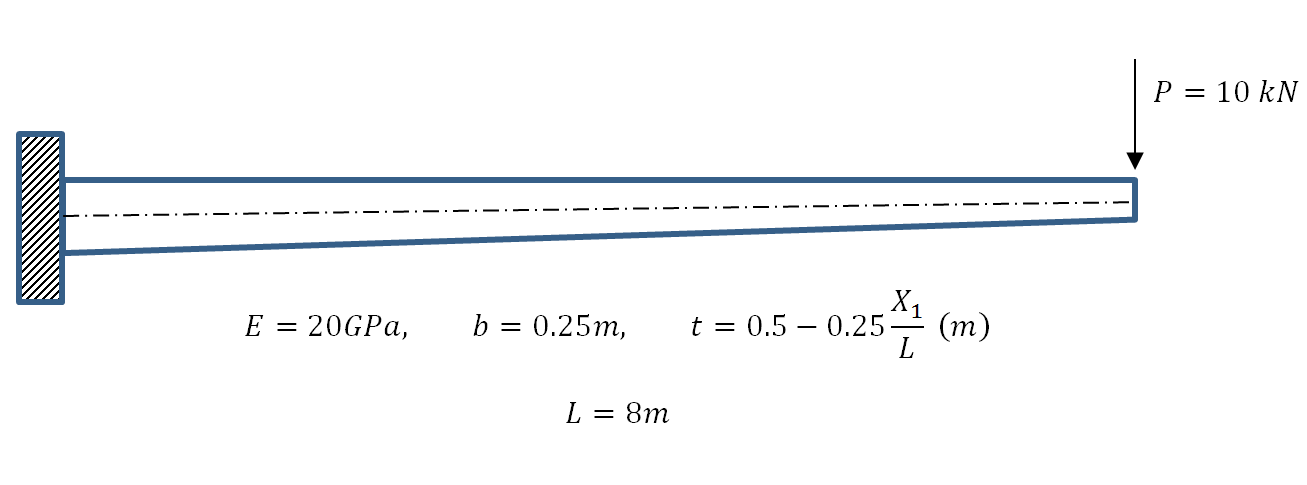
Example 3: Cantilever Beam with a Varying Cross Sectional Area

Let a beam with a length $L=8m$ and with a constant width $b=0.25m$ and a linearly varying height ( $@X_1=0, h=0.5m$ and $@X_1=8, h=0.25m$ ) be aligned with the coordinate axis $X_1$ . Assume that the beam has a fixed left end and had a shearing load acting downwards of 10kN on its right end. Find the displacement, bending moment, and shearing force on the beam by directly solving the differential equation of equilibrium and then using the Rayleigh Ritz method assuming polynomials of the degrees (0, 1, 2, 3, 4, 5, 6, 7). Assume the beam to be linear elastic with Young’s modulus $E= 20 GPa$ and that the Euler Bernoulli Beam is an appropriate beam approximation. Compare the Rayleigh Ritz method with the exact solution.

Solution

Exact Solution: First, the exact solution that would satisfy the equilibrium equations can be obtained. The equilibrium equation as shown in the Euler Bernoulli beam section apply only when $E$ and $I$ are constant. Since $I$ is variable, the differential equation has the form:

$\frac{\mathrm{d}^2\left(EI\frac{\mathrm{d}^2y}{\mathrm{d}X_1^2}\right)}{\mathrm{d}X_1^2}=q$

For the cantilever beam, $q=0$ . For consistency in the units, in all the following calculations $E=20,000,000,000 Pa$ and $P=10,000 N$ . The moment of inertia is a function of $X_1$ as follows:

$I=\frac{bt^3}{12}=\frac{0.25\left(0.5-0.25\frac{X_1}{8}\right)^3}{12}=\frac{(16-X_1)^3}{1572864}$

The exact solution can be obtained using Mathematica. The following are the four boundary conditions required:

$\begin{split} & @X_1=0:y=0\\ & @X_1=0:\theta=\frac{\mathrm{d}y}{\mathrm{d}X_1}=0\\ & @X_1=L:V=\frac{\mathrm{d}M}{\mathrm{d}X_1}=\frac{\mathrm{d}\left(EI\frac{\mathrm{d}^2y}{\mathrm{d}X_1^2}\right)}{\mathrm{d}X_1}=10000\\ & @X_1=L:M=EI\frac{\mathrm{d}^2y}{\mathrm{d}X_1^2}=0\\ \end{split}$

Using Mathematica, the above differential equation can be solved to yield the following exact solution for $y$ :

$y=\frac{34.8872+(0.036864X_1-2.96688)X_1+(0.786432X_1-12.5829)\ln[16-X_1]}{X_1-16}$

The associated moment in N.m. and shearing force in N. are given by:

$M=-80000+10000X_1\qquad V=10000$

Obviously, as the beam is statically determinate, the equations for the moment and shear are very simple. However, the variable cross section leads to a complicated form for the displacement $y$ . Note that traditionally, in structural engineering applications, a constant cross section with the intermediate height of two thirds of the maximum height can be assumed to simplify the equations.

The Rayleigh Ritz Method:
The first step in the Rayleigh Ritz method finds the minimizer of the potential energy of the system which can be written as:

$PE=\int\!\overline{U}\,dX - W=\int_0^L\!\frac{EI}{2}\left(\frac{\mathrm{d}^2y}{\mathrm{d}X_1^2}\right)^2 \,\mathrm{d}X_1 - (-P)y|_{X_1=L}$

Notice that the potential energy lost by the action of the end force $P$ is equal to the product of - $P$ ( $P$ is acting downwards and y is assumed upwards) and the displacement $y$ evaluated at $X_1= L$ . To find an approximate solution, an assumption for the shape or the form of $y$ has to be introduced.
Polynomials of the Zero and First Degrees:
If we assume that $y$ is a constant (polynomial of the zero degree) or a linear (polynomial of the first degree) function, and when attempting to satisfy the essential boundary conditions:

$\begin{split} @X_1=0 & :y=0\\ @X_1=0 & :\theta=\frac{\mathrm{d}y}{\mathrm{d}X_1}=0 \end{split}$

this leads to the trivial solution $y= 0$ , which will automatically be rejected.

$\begin{split} y & =a_2X_1^2+a_1X_1+a_0\\ \theta &=\frac{\mathrm{d}y}{\mathrm{d}X_1} =2a_2X_1+a_1\\ M &=EI\frac{\mathrm{d}^2y}{\mathrm{d}X_1^2} =2EIa_2=-\frac{9765625}{384}a_2(-16+X_1)^3\\ V &=\frac{\mathrm{d}M}{\mathrm{d}X_1}=-\frac{9765625}{128}a_2(-16+X_1)^2 \end{split}$

To satisfy the essential boundary conditions, we have:

$\begin{split} @X_1=0 & :y=0\Rightarrow a_0=0\\ @X_1=0 & :\theta=\frac{\mathrm{d}y}{\mathrm{d}X_1}=0\Rightarrow a_1=0 \end{split}$

Therefore, the solutions forms have only one parameter $a_2$ that can be controlled:

$\begin{split} y & =a_2X_1^2\\ \theta &=\frac{\mathrm{d}y}{\mathrm{d}X_1} =2a_2X_1\\ M &=EI\frac{\mathrm{d}^2y}{\mathrm{d}X_1^2} =2EIa_2=-\frac{9765625}{384}a_2(-16+X_1)^3\\ V &=\frac{\mathrm{d}M}{\mathrm{d}X_1}=-\frac{9765625}{128}a_2(-16+X_1)^2 \end{split}$

Substituting into the equation of the potential energy of an Euler Bernoulli beam:

$\begin{split} PE&=\int_0^L\!\frac{EI}{2} \left(2a_2\right)^2\,\mathrm{d}X_1+P\left(a_2L^2\right)=\int_0^L\!\frac{9765625a_2^2(16-X_1)^3}{384}\,\mathrm{d}X_1+640000a_2\\ &=640000a_2+390625000a_2^2 \end{split}$

Note that $I$ is a function of $X_1$ and so it stays inside the integral. The unknown coefficient $a_2$ can be obtained by minimizing the potential energy:

$\frac{\mathrm{d} PE}{\mathrm{d} a_2} =0\Rightarrow a_2=\frac{-64}{78125}$

Therefore, the “best” parabolic approximation for $y$ along with the corresponding solutions for $M$ and $V$ are given by:

$\begin{split} y & =\frac{-64}{78125}X_1^2=-0.0008192X_1^2\\ M &=EI\frac{\mathrm{d}^2y}{\mathrm{d}X_1^2} =\frac{125}{6}(X_1-16)^3\\ &=-85333.3 + 16000 X_1 - 1000 X_1^2 + 20.8333 X_1^3\\ V &=\frac{\mathrm{d}M}{\mathrm{d}X_1} =\frac{125}{2}(X_1-16)^2\\ &=16000 - 2000 X_1 + 62.5 X_1^2 \end{split}$

To satisfy the essential boundary conditions, we have:

$\begin{split} @X_1=0 & :y=0\Rightarrow a_0=0\\ @X_1=0 & :\theta=\frac{\mathrm{d}y}{\mathrm{d}X_1}=0\Rightarrow a_1=0 \end{split}$

Therefore, the solutions forms have only two parameters $a_2$ and $a_3$ that can be controlled:

$\begin{split} y & =a_3X_1^3+a_2X_1^2\\ \theta &=\frac{\mathrm{d}y}{\mathrm{d}X_1} =3a_3X_1^2+2a_2X_1\\ M &=EI\frac{\mathrm{d}^2y}{\mathrm{d}X_1^2} =6EIa_3X_1+2EIa_2=-\frac{9765625}{384}(-16+X_1)^3(a_2+3a_3X_1)\\ V &=-\frac{9765625}{128}(-16+X_1)^2(a_2+4a_3(X_1-4)) \end{split}$

Substituting into the equation of the potential energy of an Euler Bernoulli beam:

$PE=\int_0^L\!\frac{EI}{2}\left(6a_3X_1+2a_2\right)^2\,\mathrm{d}X_1+P\left(a_3L^3+a_2L^2\right)$

The unknown coefficients $a_2$ and $a_3$ can be obtained by minimizing the potential energy:

$\begin{split} \frac{\partial PE}{\partial a_2} & =640000+781250000a_2+6500000000a_3=0\\ \frac{\partial PE}{\partial a_3} & =5120000+6500000000a_2+84000000000a_3=0 \end{split}$

Solving the above two equations yields:

$a_2=-\frac{512}{584375} \qquad a_3=\frac{4}{584375}$

Therefore, the “best” cubic approximation for $y$ along with the corresponding solutions for $\theta, M$ , and $V$ are given by:

$\begin{split} y & =\frac{4X_1^3}{584375}-\frac{512X_1^2}{584375}\\ &=-0.00087615X_1^2+6.84492(10)^{-6}X_1^3\\ M &=EI\frac{\mathrm{d}^2y}{\mathrm{d}X_1^2} =-\frac{3125(-16+X_1)^3(-128+3X_1)}{17952}\\ &=-91265.6 + 19251.3 X_1 - 1470.59 X_1^2 + 47.3485 X_1^3 - 0.522226 X_1^4\\ V &=\frac{\mathrm{d}M}{\mathrm{d}X_1} =-\frac{3125(-36+X_1)(-16+X_1)^2}{1496}\\ &=19251.3 - 2941.18 X_1 + 142.045 X_1^2 - 2.0889 X_1^3 \end{split}$

Polynomials of the Fourth Degree:
The approximate solution forms for the displacement $y$ , the rotation $\theta$ , the moment $M$ , and the shear force $V$ functions if $y$ is assumed to be a polynomial of the fourth degree are:

To satisfy the essential boundary conditions, we have:

$\begin{split} @X_1=0 & :y=0\Rightarrow a_0=0\\ @X_1=0 & :\theta=\frac{\mathrm{d}y}{\mathrm{d}X_1}=0\Rightarrow a_1=0 \end{split}$

Therefore, the solutions forms have the parameters $a_2, a_3$ , and $a_4$ that can be controlled:

$\begin{split} y & =a_4X_1^4+a_3X_1^3+a_2X_1^2\\ M &=EI\frac{\mathrm{d}^2y}{\mathrm{d}X_1^2} =12EIa_4X_1^2+6EIa_3X_1+2EIa_2\\ V &=\frac{\mathrm{d}M}{\mathrm{d}X_1} \end{split}$

Substituting into the equation of the potential energy of an Euler Bernoulli beam:

$PE=\int_0^L\!\frac{EI}{2}\left(12a_4X_1^2+6a_3X_1+2a_2\right)^2\,\mathrm{d}X_1+P\left(a_4L^4+a_3L^3+a_2L^2\right)$

The unknown coefficients $a_2, a_3$ , and $a_4$ can be obtained by minimizing the potential energy:

$\frac{\partial PE}{\partial a_2} =0\qquad \frac{\partial PE}{\partial a_3} =0 \qquad \frac{\partial PE}{\partial a_4} =0$

Solving the above three equations yields:

$a_2=-0.000704051 \qquad a_3=-0.0000484584 \qquad a_4=-4.01821(10)^{-6}$

Therefore, assuming a fourth order polynomial gives the following set of solutions:

$\begin{split} y & =-0.000704051X_1^2-0.0000484584X_1^3+4.01821(10)^{-6}X_1^4\\ M &=EI\frac{\mathrm{d}^2y}{\mathrm{d}X_1^2} =-73338.7 - 1392.24 X_1 + 4491.3 X_1^2 - 630.438 X_1^3 + 33.1273 X_1^4 - 0.61313 X_1^5\\ V &=\frac{\mathrm{d}M}{\mathrm{d}X_1}=-1392.24 + 8982.6 X_1 - 1891.32 X_1^2 + 132.509 X_1^3 - 3.06565 X_1^4 \end{split}$

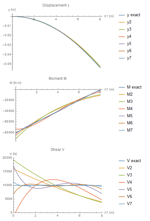
Approximate solutions using higher order polynomials can be obtained similarly. The following plots show the convergence of the polynomial functions to the exact solution up to a polynomial of the sixth degree (Mathematica code is given below). In the first plot, it is clear that a polynomial of the second degree is capable of capturing the displacement quite accurately. However, the corresponding approximate solutions for the moment and shear are not as accurate. The accuracy of the approximate solution for the bending moment is higher than that for the shearing force and that is because the moment is related to the second derivative of $y$ while the shear is related to the third derivative of $y$ . It takes up to a polynomial of the seventh degree for $y$ for the approximate shearing force to have a flat distribution similar to the exact solution.

View Mathematica Code

Clear[y, b, L, t, Ii, Ee, P]
b = 1/4;
L = 8;
t = (1/2 - 1/4*X1/L);
Ii = b*t^3/12;
Ee = 20*10^9;
P = 10000;
a = DSolve[{D[Ee*Ii*y''[X1], {X1, 2}] == 0, y[0] == 0, y'[0] == 0, y''[L] == 0, (D[Ee*Ii, X1] /. X1 -> L)*y''[L] + (Ee*Ii /. X1 -> L)*y'''[L] == P}, y[X1], X1, Assumptions -> 0 <= X1 <= L]
y = FullSimplify[Chop[N[y[X1] /. a[[1]]]]]
th = D[y, X1];
M = FullSimplify[Ee*Ii*D[y, {X1, 2}]]
V = FullSimplify[D[M, X1]]
Plot[y, {X1, 0, L}, PlotLabel -> "Displacement y", AxesLabel -> {"X1 (m)", "y (m)"}, PlotLegends -> {"y exact"}]
Plot[M, {X1, 0, L}, PlotLabel -> "Moment M", AxesLabel -> {"X1 (m)", "M (N.m)"}, PlotLegends -> {"M exact"}]
Plot[V, {X1, 0, L}, PlotRange -> {{0, L}, {0, 2 P}}, PlotLabel -> "Shear V", AxesLabel -> {"X1 (m)", "V (N)"}, PlotLegends -> {"V exact"}]
Print["Second Order Polynomial"]
y2 = a2*X1^2;
d2y = D[y2, {X1, 2}];
PE = Integrate[Ee*Ii/2*d2y^2, {X1, 0, L}] - (-P)*y2 /. X1 -> L;
sol = Solve[D[PE, a2] == 0, a2]
y2 = y2 /. sol[[1]]
M2 = FullSimplify[Ee*Ii*D[y2, {X1, 2}]]
V2 = FullSimplify[D[M2, X1]]
Plot[{y, y2}, {X1, 0, L}, PlotLabel -> "Displacement y", AxesLabel -> {"X1 (m)", "y (m)"}, PlotLegends -> {"y exact", "y2"}]
Plot[{M, M2}, {X1, 0, L}, PlotLabel -> "Moment M", AxesLabel -> {"X1 (m)", "M (N.m)"}, PlotLegends -> {"M exact", "M2"}]
Plot[{V, V2}, {X1, 0, L}, PlotRange -> {{0, L}, {0, 2 P}}, PlotLabel -> "Shear V", AxesLabel -> {"X1 (m)", "V (N)"}, PlotLegends -> {"V exact", "V2"}]
Print["Third Order Polynomial"]
y3 = a2*X1^2 + a3*X1^3;
d2y = D[y3, {X1, 2}];
PE = Integrate[Ee*Ii/2*d2y^2, {X1, 0, L}] - (-P)*y3 /. X1 -> L;
sol = Solve[{D[PE, a2] == 0, D[PE, a3] == 0}, {a2, a3}]
y3 = y3 /. sol[[1]]
M3 = FullSimplify[Ee*Ii*D[y3, {X1, 2}]]
V3 = FullSimplify[D[M3, X1]]
Plot[{y, y3}, {X1, 0, L}, PlotLabel -> "Displacement y", AxesLabel -> {"X1 (m)", "y (m)"}, PlotLegends -> {"y exact", "y3"}]
Plot[{M, M3}, {X1, 0, L}, PlotLabel -> "Moment M", AxesLabel -> {"X1 (m)", "M (N.m)"}, PlotLegends -> {"M exact", "M3"}]
Plot[{V, V3}, {X1, 0, L}, PlotRange -> {{0, L}, {0, 2 P}}, PlotLabel -> "Shear V", AxesLabel -> {"X1 (m)", "V (N)"}, PlotLegends -> {"V exact", "V3"}]
Print["Fourth Order Polynomial"]
y4 = a2*X1^2 + a3*X1^3 + a4*X1^4;
d2y = D[y4, {X1, 2}];
PE = Integrate[Ee*Ii/2*d2y^2, {X1, 0, L}] - (-P)*y4 /. X1 -> L;
sol = Solve[{D[PE, a2] == 0, D[PE, a3] == 0, D[PE, a4] == 0}, {a2, a3, a4}]
y4 = y4 /. sol[[1]]
M4 = FullSimplify[Ee*Ii*D[y4, {X1, 2}]]
V4 = FullSimplify[D[M4, X1]]
Plot[{y, y4}, {X1, 0, L}, PlotLabel -> "Displacement y", AxesLabel -> {"X1 (m)", "y (m)"}, PlotLegends -> {"y exact", "y4"}]
Plot[{M, M4}, {X1, 0, L}, PlotLabel -> "Moment M", AxesLabel -> {"X1 (m)", "M (N.m)"}, PlotLegends -> {"M exact", "M4"}]
Plot[{V, V4}, {X1, 0, L}, PlotRange -> {{0, L}, {0, 2 P}}, PlotLabel -> "Shear V", AxesLabel -> {"X1 (m)", "V (N)"}, PlotLegends -> {"V exact", "V4"}]
Print["Fifth Order Polynomial"]
y5 = a2*X1^2 + a3*X1^3 + a4*X1^4 + a5*X1^5;
d2y = D[y5, {X1, 2}];
PE = Integrate[Ee*Ii/2*d2y^2, {X1, 0, L}] - (-P)*y5 /. X1 -> L; sol = Solve[{D[PE, a2] == 0, D[PE, a3] == 0, D[PE, a4] == 0, D[PE, a5] == 0}, {a2, a3, a4, a5}]
y5 = y5 /. sol[[1]]
M5 = FullSimplify[Ee*Ii*D[y5, {X1, 2}]]
V5 = FullSimplify[D[M5, X1]]
Plot[{y, y5}, {X1, 0, L}, PlotLabel -> "Displacement y", AxesLabel -> {"X1 (m)", "y (m)"}, PlotLegends -> {"y exact", "y5"}]
Plot[{M, M5}, {X1, 0, L}, PlotLabel -> "Moment M", AxesLabel -> {"X1 (m)", "M (N.m)"}, PlotLegends -> {"M exact", "M5"}]
Plot[{V, V5}, {X1, 0, L}, PlotRange -> {{0, L}, {0, 2 P}}, PlotLabel -> "Shear V", AxesLabel -> {"X1 (m)", "V (N)"}, PlotLegends -> {"V exact", "V5"}]
Print["Sixth Order Polynomial"]
y6 = a2*X1^2 + a3*X1^3 + a4*X1^4 + a5*X1^5 + a6*X1^6;
d2y = D[y6, {X1, 2}];
PE = Integrate[Ee*Ii/2*d2y^2, {X1, 0, L}] - (-P)*y6 /. X1 -> L; sol = Solve[{D[PE, a2] == 0, D[PE, a3] == 0, D[PE, a4] == 0, D[PE, a5] == 0, D[PE, a6] == 0}, {a2, a3, a4, a5, a6}]
y6 = y6 /. sol[[1]]
M6 = FullSimplify[Ee*Ii*D[y6, {X1, 2}]]
V6 = FullSimplify[D[M6, X1]]
Plot[{y, y6}, {X1, 0, L}, PlotLabel -> "Displacement y", AxesLabel -> {"X1 (m)", "y (m)"}, PlotLegends -> {"y exact", "y6"}]
Plot[{M, M6}, {X1, 0, L}, PlotLabel -> "Moment M", AxesLabel -> {"X1 (m)", "M (N.m)"}, PlotLegends -> {"M exact", "M6"}]
Plot[{V, V6}, {X1, 0, L}, PlotRange -> {{0, L}, {0, 2 P}}, PlotLabel -> "Shear V", AxesLabel -> {"X1 (m)", "V (N)"}, PlotLegends -> {"V exact", "V6"}]
Print["Seventh Order Polynomial"]
y7 = a2*X1^2 + a3*X1^3 + a4*X1^4 + a5*X1^5 + a6*X1^6 + a7*X1^7; d2y = D[y7, {X1, 2}];
PE = Integrate[Ee*Ii/2*d2y^2, {X1, 0, L}] - (-P)*y7 /. X1 -> L;
sol = Solve[{D[PE, a2] == 0, D[PE, a3] == 0, D[PE, a4] == 0, D[PE, a5] == 0, D[PE, a6] == 0, D[PE, a7] == 0}, {a2, a3, a4, a5,a6, a7}]
y7 = y7 /. sol[[1]]
M7 = FullSimplify[Ee*Ii*D[y7, {X1, 2}]]
V7 = FullSimplify[D[M7, X1]]
Plot[{y, y7}, {X1, 0, L}, PlotLabel -> "Displacement y", AxesLabel -> {"X1 (m)", "y (m)"}, PlotLegends -> {"y exact", "y7"}]
Plot[{M, M7}, {X1, 0, L}, PlotLabel -> "Moment M", AxesLabel -> {"X1 (m)", "M (N.m)"}, PlotLegends -> {"M exact", "M7"}]
Plot[{V, V7}, {X1, 0, L}, PlotRange -> {{0, L}, {0, 2 P}}, PlotLabel -> "Shear V", AxesLabel -> {"X1 (m)", "V (N)"}, PlotLegends -> {"V exact", "V7"}]
Plot[{y, y2, y3, y4, y5, y6, y7}, {X1, 0, L}, PlotLabel -> "Displacement y", AxesLabel -> {"X1 (m)", "y (m)"}, PlotLegends -> {"y exact", "y2", "y3", "y4", "y5", "y6", "y7"}]
Plot[{M, M2, M3, M4, M5, M6, M7}, {X1, 0, L}, PlotLabel -> "Moment M", AxesLabel -> {"X1 (m)", "M (N.m)"}, PlotLegends -> {"M exact", "M2", "M3", "M4", "M5", "M6", "M7"}]
Plot[{V,V2,V3,V4,V5,V6,V7}, {X1, 0, L}, PlotRange ->{{0, L}, {0, 2 P}},PlotLabel->"Shear V",AxesLabel -> {"X1 (m)", "V (N)"},PlotLegends -> {"V exact", "V2", "V3", "V4", "V5", "V6", "V7"}]

View Python Code

from sympy import *
from numpy import *
import sympy as sp 
import numpy as np
import matplotlib.pyplot as plt
sp.init_printing(use_latex = "mathjax")
x, a2, a3, a4, a5, a6, a7, EI, L, E= symbols("x a_2 a_3 a_4 a_5 a_6 a_7 EI L E")
display("Exact")
b = 1/4
L = 8
t = (1/2-1/4*x/L)
I = b*t**3/12
E = 20*10**9
P = 10000
# Exact solution done in mathematica code
y = (34.8872 + (-2.96688 + 0.036864*x)*x + (-12.5829 + 0.786432*x)*sp.ln(16-x))/(x-16)
M = -80000 + 10000*x
V = M.diff(x)
display("y,M,V: ", y, M, V)
display("Second Order Polynomial")
y2 = a2*x**2
d2y = y2.diff(x,2)
PE2 = integrate(E*I/2*d2y**2, (x,0,L)) - (-P)*y2.subs(x,L)
display("Potential Energy: ", PE2)
sol = solve(PE2.diff(a2), a2)
y2 = y2.subs(a2,sol[0])
M2 = E*I*y2.diff(x,2)
V2 = M2.diff(x)
display("y2,M2,V2: ", y2, M2, V2)
display("Third Order Polynomial")
y3 = a2*x**2+a3*x**3
d2y = y3.diff(x,2)
PE3 = integrate(E*I/2*d2y**2, (x,0,L)) - (-P)*y3.subs(x,L)
display("Potential Energy: ", PE3)
sol = solve((PE3.diff(a2), PE3.diff(a3)), (a2,a3))
y3 = y3.subs({a2:sol[a2], a3:sol[a3]})
M3 = E*I*y3.diff(x,2)
V3 = M3.diff(x)
display("y3,M3,V3: ", y3, M3, V3)
display("Fourth Order Polynomial")
y4 = a2*x**2+a3*x**3+a4*x**4
d2y = y4.diff(x,2)
PE4 = integrate(E*I/2*d2y**2, (x,0,L)) - (-P)*y4.subs(x,L)
display("Potential Energy: ", PE4)
sol = solve((PE4.diff(a2), PE4.diff(a3), PE4.diff(a4)), (a2,a3,a4))
y4 = y4.subs({a2:sol[a2], a3:sol[a3], a4:sol[a4]})
M4 = E*I*y4.diff(x,2)
V4 = M4.diff(x)
display("y4,M4,V4: ", y4, M4, V4)
display("Fifth Order Polynomial")
y5 = a2*x**2+a3*x**3+a4*x**4+a5*x**5
d2y = y5.diff(x,2)
PE5 = integrate(E*I/2*d2y**2, (x,0,L)) - (-P)*y5.subs(x,L)
display("Potential Energy: ", PE5)
sol = solve((PE5.diff(a2), PE5.diff(a3), PE5.diff(a4), PE5.diff(a5)), (a2,a3,a4,a5))
y5 = y5.subs({a2:sol[a2], a3:sol[a3], a4:sol[a4], a5:sol[a5]})
M5 = E*I*y5.diff(x,2)
V5 = M5.diff(x)
display("y5,M5,V5: ", y5, M5, V5)
display("Sixth Order Polynomial")
y6 = a2*x**2+a3*x**3+a4*x**4+a5*x**5+a6*x**6
d2y = y6.diff(x,2)
PE6 = integrate(E*I/2*d2y**2, (x,0,L)) - (-P)*y6.subs(x,L)
display("Potential Energy: ", PE6)
sol = solve((PE6.diff(a2), PE6.diff(a3), PE6.diff(a4), PE6.diff(a5), PE6.diff(a6)), (a2,a3,a4,a5,a6))
y6 = y6.subs({a2:sol[a2], a3:sol[a3], a4:sol[a4], a5:sol[a5], a6:sol[a6]})
M6 = E*I*y6.diff(x,2)
V6 = M6.diff(x)
display("y6,M6,V6: ", y6, M6, V6)
display("Seventh Order Polynomial")
y7 = a2*x**2+a3*x**3+a4*x**4+a5*x**5+a6*x**6+a7*x**7
d2y = y7.diff(x,2)
PE7 = integrate(E*I/2*d2y**2, (x,0,L)) - (-P)*y7.subs(x,L)
display("Potential Energy: ", PE7)
sol = solve((PE7.diff(a2), PE7.diff(a3), PE7.diff(a4), PE7.diff(a5), PE7.diff(a6), PE7.diff(a7)), (a2,a3,a4,a5,a6,a7))
y7 = y7.subs({a2:sol[a2], a3:sol[a3], a4:sol[a4], a5:sol[a5], a6:sol[a6], a7:sol[a7]})
M7 = E*I*y7.diff(x,2)
V7 = M7.diff(x)
display("y7,M7,V7: ", y7, M7, V7)
#Graph
fig, ax = plt.subplots(3,1, figsize = (10,15))
plt.setp(ax[0], xlabel = "x(m) ", ylabel = "y(m)")
plt.setp(ax[1], xlabel = "x(m)", ylabel = "M(N*m)")
plt.setp(ax[2], xlabel = "x(m)", ylabel = "V(N)")
x1 = np.arange(0,8.1,0.1)
y_list = [y.subs({x:i}) for i in x1]
y2_list = [y2.subs({x:i}) for i in x1]
y3_list = [y3.subs({x:i}) for i in x1]
y4_list = [y4.subs({x:i}) for i in x1]
y5_list = [y5.subs({x:i}) for i in x1]
y6_list = [y6.subs({x:i}) for i in x1]
y7_list = [y7.subs({x:i}) for i in x1]
M_list = [M.subs({x:i}) for i in x1]
M2_list = [M2.subs({x:i}) for i in x1]
M3_list = [M3.subs({x:i}) for i in x1]
M4_list = [M4.subs({x:i}) for i in x1]
M5_list = [M5.subs({x:i}) for i in x1]
M6_list = [M6.subs({x:i}) for i in x1]
M7_list = [M7.subs({x:i}) for i in x1]
V_list = [V.subs({x:i}) for i in x1]
V2_list = [V2.subs({x:i}) for i in x1]
V3_list = [V3.subs({x:i}) for i in x1]
V4_list = [V4.subs({x:i}) for i in x1]
V5_list = [V5.subs({x:i}) for i in x1]
V6_list = [V6.subs({x:i}) for i in x1]
V7_list = [V7.subs({x:i}) for i in x1]
ax[0].plot(x1, y_list, 'blue', label = "Exact y")
ax[0].plot(x1, y2_list, 'orange', label = "y2")
ax[0].plot(x1, y3_list, 'green', label = "y3")
ax[0].plot(x1, y4_list, 'red', label = "y4")
ax[0].plot(x1, y5_list, 'purple', label = "y5")
ax[0].plot(x1, y6_list, 'brown', label = "y6")
ax[0].plot(x1, y7_list, 'cyan', label = "y7")
ax[0].legend()
ax[1].plot(x1, M_list, 'blue', label = "Exact M")
ax[1].plot(x1, M2_list, 'orange', label = "y2")
ax[1].plot(x1, M3_list, 'green', label = "y3")
ax[1].plot(x1, M4_list, 'red', label = "y4")
ax[1].plot(x1, M5_list, 'purple', label = "y5")
ax[1].plot(x1, M6_list, 'brown', label = "y6")
ax[1].plot(x1, M7_list, 'cyan', label = "y7")
ax[1].legend()
ax[2].plot(x1, V_list, 'blue', label = "Exact V")
ax[2].plot(x1, V2_list, 'orange', label = "y2")
ax[2].plot(x1, V3_list, 'green', label = "y3")
ax[2].plot(x1, V4_list, 'red', label = "y4")
ax[2].plot(x1, V5_list, 'purple', label = "y5")
ax[2].plot(x1, V6_list, 'brown', label = "y6")
ax[2].plot(x1, V7_list, 'cyan', label = "y7")
ax[2].legend()