Engineering at Alberta Courses » Illustrative Examples for the Principle of Virtual Work

The Principle of Virtual Work: Illustrative Examples for the Principle of Virtual Work

Learning Outcomes

Describe the different expressions that appear in the statement of virtual work in a continuum.
Describe the different expressions that appear in the statement of virtual work in an Euler Bernoulli beam.

Example 1: Illustrative Example of the Principle of Virtual Work Applied to a Continuum

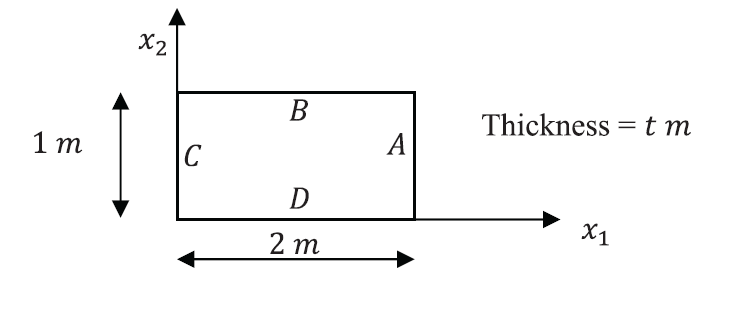
The Cauchy stress distribution in the shown plate is given by:

$\sigma=\left(\begin{matrix}x_1x_2&5&0\\5&x_1&0\\0&0&0\end{matrix}\right)KN/m^2$

where $x_1$ and $x_2$ are the coordinates inside the plate with units of $m$ . Find the equilibrium body forces vector applied to the plate. Find the traction forces on the boundary edges $A$ , $B$ , $C$ , and $D$ of the plate. Verify the principle of virtual work assuming a virtual displacement field $u_1^*=ax_1+bx_2, a,b>0$ .

SOLUTION:

The equilibrium body forces applied to the plate can be obtained using the equilibrium equations:

$\begin{split} \rho b_1 & =-\frac{\partial \sigma_{11}}{\partial x_1}-\frac{\partial \sigma_{21}}{\partial x_2}-\frac{\partial \sigma_{31}}{\partial x_3}=-x_2\\ \rho b_2 & =-\frac{\partial \sigma_{12}}{\partial x_1}-\frac{\partial \sigma_{22}}{\partial x_2}-\frac{\partial \sigma_{32}}{\partial x_3}=0\\ \rho b_3 & =-\frac{\partial \sigma_{13}}{\partial x_1}-\frac{\partial \sigma_{23}}{\partial x_2}-\frac{\partial \sigma_{33}}{\partial x_3}=0 \end{split}$

The plate is in a state of plane stress, so, the problem can be reduced to $\mathbb{R}^2$ . The area vectors for the boundary edges $A, B, C$ , and $D$ are given by:

$n_A=\left(\begin{array}{c}1\\0\end{array}\right) \qquad n_B=\left(\begin{array}{c}0\\1\end{array}\right) \qquad n_C=\left(\begin{array}{c}-1\\0\end{array}\right) \qquad n_D=\left(\begin{array}{c}0\\-1\end{array}\right)$

The traction vectors in units of $KN/m^2$ on the boundary edges $A$ , $B$ , $C$ , and $D$ are given by:

$t_A=(\sigma^Tn_A)|_{x_1=2} \qquad t_B=(\sigma^Tn_B)|_{x_2=1} \qquad t_C=(\sigma^Tn_C)|_{x_1=0} \qquad t_D=(\sigma^Tn_D)|_{x_2=0}$

Therefore,

$t_A=\left(\begin{array}{c}2x_2\\5\end{array}\right)\qquad t_B=\left(\begin{array}{c}5\\x_1\end{array}\right)\qquad t_C=\left(\begin{array}{c}0\\-5\end{array}\right)\qquad t_D=\left(\begin{array}{c}-5\\-x_1\end{array}\right)$

The virtual displacement vector is:

$u^*=\left(\begin{array}{c}ax_1+bx_2\\0\end{array}\right)$

The gradient of the virtual displacement tensor is:

$\nabla u^*=\left(\begin{array}{cc}a & b\\0 & 0\end{array}\right)$

The associated virtual strain is given by:

$\varepsilon^*=\frac{1}{2}\left(\nabla u^*+\nabla (u^*)^T\right)=\left(\begin{array}{cc}a & \frac{b}{2}\\\frac{b}{2} & 0\end{array}\right)$

The internal virtual work can be calculated as follows:

$IVW=\int_0^t \int_0^1 \int_0^2 \! \sum_{i,j=1}^3\sigma_{ij}\varepsilon_{ij}^*\,\mathrm{d}x_1\mathrm{d}x_2\mathrm{d}x_3=\int_0^t \int_0^1 \int_0^2 \! 5b+ax_1x_2\,\mathrm{d}x_1\mathrm{d}x_2\mathrm{d}x_3=(a+10b)t$

There are five components for the external virtual work. The first one is the external virtual work due to the external body forces applied to the plate. This component is a volume integral:

$\begin{split} EVW|_{\mbox{Body Forces}}&=\int_0^t \int_0^1 \int_0^2 \! \sum_{i}^3\rho b_i u_i^* \,\mathrm{d}x_1\mathrm{d}x_2\mathrm{d}x_3\\ &=\int_0^t \int_0^1 \int_0^2 \! -x_2(ax_1+bx_2)\,\mathrm{d}x_1\mathrm{d}x_2\mathrm{d}x_3\\ &=-\frac{1}{3}(3a+2b)t \end{split}$

The second component is the external virtual work due to the external forces acting on side $A$ . This is a surface integral and is evaluated for side $A$ where $x_1=2$ :

$EVW|_A=\int_0^t \int_0^1 \! t_A\cdot u^*|_{x_1=2} \,\mathrm{d}x_2\mathrm{d}x_3=\int_0^t \int_0^1 \! 2 x_2 (2 a + b x_2)\,\mathrm{d}x_2\mathrm{d}x_3=2\left(a+\frac{b}{3}\right)t$

The third component is the external virtual work due to the external forces acting on side $B$ . This is a surface integral and is evaluated for side $B$ where $x_2=1$ :

$EVW|_B=\int_0^t \int_0^2 \! t_B\cdot u^*|_{x_2=1} \,\mathrm{d}x_1\mathrm{d}x_3=\int_0^t \int_0^2 \! 5 (b + a x_1)\,\mathrm{d}x_1\mathrm{d}x_3=10\left(a+b\right)t$

The fourth component is the external virtual work due to the external forces acting on side $C$ . This is a surface integral and is evaluated for side $C$ where $x_1=0$ :

$EVW|_C=\int_0^t \int_0^1 \! t_C\cdot u^*|_{x_1=0} \,\mathrm{d}x_2\mathrm{d}x_3=\int_0^t \int_0^1 \! 0\,\mathrm{d}x_2\mathrm{d}x_3=0$

The fifth component is the external virtual work due to the external forces acting on side $D$ . This is a surface integral and is evaluated for side $D$ where $x_2=0$ :

$EVW|_D=\int_0^t \int_0^2 \! t_D\cdot u^*|_{x_2=0} \,\mathrm{d}x_1\mathrm{d}x_3=\int_0^t \int_0^2 \! -5ax_1\,\mathrm{d}x_1\mathrm{d}x_3=-10at$

Therefore, the total external virtual work is:

$\begin{split} EVW & =EVW_{\mbox{Body Forces}}+EVW_A+EVW_B+EVW_C+EVW_D\\ & =-\frac{1}{3}(3a+2b)t+2\left(a+\frac{b}{3}\right)t+10\left(a+b\right)t+0-10at\\ & =(a+10b)t\\ & =IVW \end{split}$

View Mathematica Code

s = {{x1*x2, 5, 0}, {5, x1, 0}, {0, 0, 0}};
x = {x1, x2, x3};
rhob1 = -Sum[D[s[[j, 1]], x[[j]]], {j, 1, 2}]
rhob2 = -Sum[D[s[[j, 2]], x[[j]]], {j, 1, 2}]
rhob3 = -Sum[D[s[[j, 3]], x[[j]]], {j, 1, 2}]
(*We will only consider the 2 dimensional matrices as all out of plane components are equal to 0*)
ustar = {a*x1 + b*x2, 0};
ustara = ustar /. x1 -> 2;
ustarb = ustar /. x2 -> 1;
ustarc = ustar /. x1 -> 0;
ustard = ustar /. x2 -> 0;
s = {{x1*x2, 5}, {5, x1}};
na = {1, 0};
nb = {0, 1};
nc = {-1, 0};
nd = {0, -1};
ta = s . na /. x1 -> 2
tb = s . nb /. x2 -> 1
tc = s . nc /. x1 -> 0
td = s . nd /. x2 -> 0
Gradustar = Table[D[ustar[[i]], x[[j]]], {i, 1, 2}, {j, 1, 2}]
estar = 1/2*(Gradustar + Transpose[Gradustar])
ststrain = Sum[s[[i, j]]*estar[[i, j]], {i, 1, 2}, {j, 1, 2}]
IVW = Integrate[ststrain, {x1, 0, 2}, {x2, 0, 1}, {x3, 0, t}]
EVWBodyForces = 
 Integrate[rhob1*ustar[[1]], {x1, 0, 2}, {x2, 0, 1}, {x3, 0, t}]
EVWa = Integrate[(ta . ustara) /. x1 -> 2, {x2, 0, 1}, {x3, 0, t}]
EVWb = Integrate[(tb . ustarb) /. x2 -> 1, {x1, 0, 2}, {x3, 0, t}]
EVWc = Integrate[(tc . ustarc) /. x1 -> 0, {x2, 0, 1}, {x3, 0, t}]
EVWd = Integrate[(td . ustard) /. x2 -> 0, {x1, 0, 2}, {x3, 0, t}]
EVW = FullSimplify[EVWBodyForces + EVWa + EVWb + EVWc + EVWd]

View PythonCode

import sympy as sp
from sympy import Matrix, diff, integrate, simplify
x1,x2,x3 = sp.symbols("x_1 x_2 x_3")
s = Matrix([[x1*x2,5,0],[5,x1,0],[0,0,0]])
x = Matrix([[x1,x2,x3]])
pb1,pb2,pb3 =[-sum([diff(s[i,j],x[i]) for i in range(3)]) for j in range(3)]
display("\u03C1b_1 =",pb1)
display("\u03C1b_2 =",pb2)
display("\u03C1b_3 =",pb3)
a,b,t = sp.symbols("a b t")
ustar = Matrix([a*x1 + b*x2, 0])
display("u* =",ustar)
gradustar = Matrix([[diff(i,j) for j in x[:2]]for i in ustar])
display("\u2207u* =",gradustar)
ustara = ustar.subs({x1:2})
ustarb = ustar.subs({x2:1})
ustarc = ustar.subs({x1:0})
ustard = ustar.subs({x2:0})
s = Matrix([[x1*x2,5],[5,x1]])
na = Matrix([1,0])
nb = Matrix([0,1])
nc = Matrix([-1,0])
nd = Matrix([0,-1])
ta = (s*na).subs({x1:2})
tb = (s*nb).subs({x2:1})
tc = (s*nc).subs({x1:0})
td = (s*nd).subs({x2:0})
display("t_A =",ta,"t_B =",tb,"t_C =",tc,"t_D =",td)
estar = sp.Rational("1/2")*(gradustar+gradustar.T)
display("\u03B5* =",estar)
ststrain = sum([s[i]*estar[i] for i in range(4)])
display("ststrain =",ststrain)
IVW = integrate(ststrain,(x1,0,2),(x2,0,1),(x3,0,t))
display("Internal Virtual Work =",IVW)
EVWBodyForces = integrate(pb1*ustar[0],(x1,0,2),(x2,0,1),(x3,0,t))
display("External Virtual Work|_{Body Forces} =",EVWBodyForces)
EVWa = integrate((ta.dot(ustara)).subs({x1:2}),(x2,0,1),(x3,0,t))
display("External Virtual Work|_A =",EVWa)
EVWb = integrate((tb.dot(ustarb)).subs({x2:1}),(x1,0,2),(x3,0,t))
display("External Virtual Work|_B =",EVWb)
EVWc = integrate((tc.dot(ustarc)).subs({x1:0}),(x2,0,1),(x3,0,t))
display("External Virtual Work|_C =",EVWc)
EVWd = integrate((td.dot(ustard)).subs({x2:0}),(x1,0,2),(x3,0,t))
display("External Virtual Work|_D =",EVWd)
EVW = simplify(EVWBodyForces+EVWa+EVWb+EVWc+EVWd)
display("External Virtual Work = Internal Virtual Work =",EVW)

Video

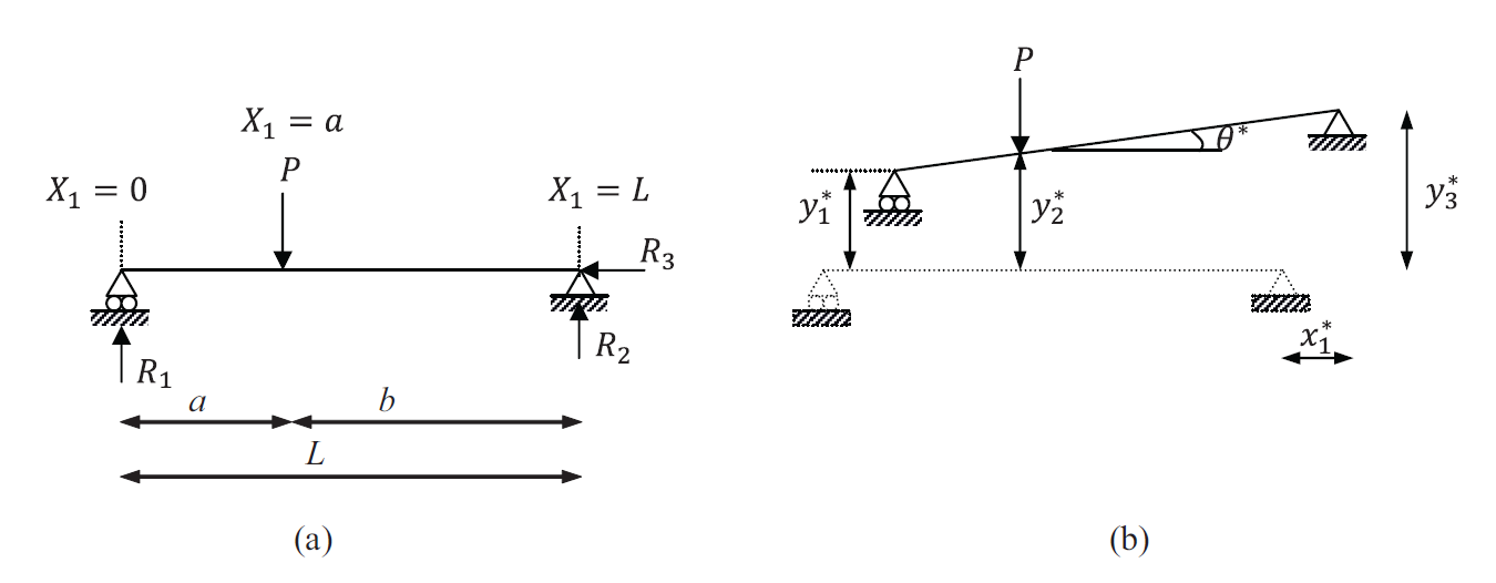
Example 2: Illustrative Example of the Principle of Virtual Work Applied to an Euler Bernoulli Beam

A fixed ends Euler Bernoulli beam is subjected to a distributed load $q=-5X_1 kN/m$ . Assuming that Young’s modulus, the length, and the moment of inertia for the beam are $E$ , $L$ , and $I$ , respectively, verify that the principle of virtual work applies when a virtual parabolic displacement $y^*=aX_1^2$ , $a>0$ is applied to the beam.

SOLUTION:

The principle of virtual work applies to the equilibrium internal forces. So, the first step is to find the internal forces at the state of equilibrium. For this, we will solve the differential equation of equilibrium:

$EI\frac{\mathrm{d}^4y}{\mathrm{d}X_1^4}=-5X_1\Rightarrow EIy=-\frac{X_1^5}{24}+\frac{C_1X_1^3}{6}+\frac{C_2X_1^2}{2}+C_3X_1+C_4$

The integration constants $C_1$ , $C_2$ , $C_3$ , and $C_4$ can be obtained using the four boundary conditions of a fixed ends beam:

$\begin{split} @X_1=0:y=0\\ @X_1=0:\theta=y'=0\\ @X_1=L:y=0\\ @X_1=L:\theta=y'=0 \end{split}$

Therefore, the equilibrium displacement of the beam is:

$y=\frac{-2L^3X_1^2+3L^2X_1^3-X_1^5}{24EI}$

The bending moment and the shearing force equations at equilibrium are:

$\begin{split} M& =EI\frac{\mathrm{d}^2y}{\mathrm{d}X_1^2}=\frac{1}{12}(-2L^3+9L^2X_1-10X_1^3)\\ V& =EI\frac{\mathrm{d}^3y}{\mathrm{d}X_1^3}=\frac{3}{4}L^2-\frac{5}{2}X_1^2 \end{split}$

The external forces acting on the ends of the beam are given by:

$M_1 =-\frac{L^3}{6}\qquad M_2=-\frac{L^3}{4} \qquad V_1=3\frac{L^2}{4}\qquad V_2=-7\frac{L^2}{4}$

Note that the convention for positive end forces is shown in Figure 3. The virtual end displacements and rotations are given by:

$y_1^*=y^*|_{X_1=0}=0 \qquad y_2^*=y^*|_{X_1=L}=aL^2\qquad \theta_1^*=\frac{\mathrm{d}y^*}{\mathrm{d}X_1}|_{X_1=0}=0\qquad \theta_2^*=\frac{\mathrm{d}y^*}{\mathrm{d}X_1}|_{X_1=L}=2aL$

Therefore, the internal virtual work is given by:

$\int_0^L \! EI \frac{\mathrm{d}^2y}{\mathrm{d}X_1^2} \frac{\mathrm{d}^2y^*}{\mathrm{d}X_1^2}\, \mathrm{d}X_1=\int_0^L \! \left(\frac{1}{12}\left(-2L^3+9L^2X_1-10X_1^3\right)\right)(2a)\, \mathrm{d}X_1 =0$

The external virtual work has three components, the first is the external virtual work due to the distributed load q:

$EVW_q= \int_0^L \! qy^* \,\mathrm{d}X_1=\int_0^L \! -5aX_1^3 \,\mathrm{d}X_1=-\frac{5aL^4}{4}$

The second component is the external virtual work due to the reactions at end 1:

$EVW_1=V_1y_1^*-M_1\theta^*_1=0$

The third component is the external virtual work due to the reactions at end 2:

$EVW_2=-V_2y_2^*+M_2\theta^*_2=\frac{5aL^4}{4}$

The total external virtual work is:

$EVW=EVW_q+EVW_1+EVW_2=-\frac{5aL^4}{4}+0+\frac{5aL^4}{4}=0=IVW$

View Mathematica Code

Clear[M, y, EI, x, s]
q = -5 x
s = DSolve[{EI*y''''[x] == q, y[0] == 0, y'[0] == 0, y[L] == 0, 
   y'[L] == 0}, y[x], x]
y = y[x] /. s[[1]]
th = D[y, x]
M = FullSimplify[EI*D[y, {x, 2}]]
V = FullSimplify[EI*D[y, {x, 3}]]
M1 = M /. x -> 0
M2 = M /. x -> L
V1 = V /. x -> 0
V2 = V /. x -> L
ystar = a*x^2;
thstar = D[ystar, x];
ystar1 = ystar /. x -> 0
ystar2 = ystar /. x -> L
thstar1 = thstar /. x -> 0
thstar2 = thstar /. x -> L
Print["IVW"]
IVW = Integrate[M*D[ystar, {x, 2}], {x, 0, L}]
EVWq = Integrate[q*ystar, {x, 0, L}]
EVW1 = +V1*ystar1 - M1*thstar1
EVW2 = -V2*ystar2 + M2*thstar2
Print["EVW"]
EVW = EVWq + EVW1 + EVW2

View Python Code

import sympy as sp
from sympy import Function,dsolve,diff,simplify,integrate
x,EI,L = sp.symbols("x EI L")
y = Function("y")
a = sp.symbols("a")
y1 = y(x).subs(x,0)
y2 = y(x).subs(x,L)
yp1 = y(x).diff(x).subs(x,0)
yp2 = y(x).diff(x).subs(x,L)
q = -5*x
s = dsolve(EI*y(x).diff(x,4)-q,y(x),ics={y1:0,y2:0,yp1:0,yp2:0})
y = s.rhs
display("y(x) =",y)
th = simplify(diff(y,x))
M = simplify(EI*diff(y,x,x))
V = simplify(EI*diff(y,x,x,x))
display("th =",th,"M =",M,"V =",V)
M1 = M.subs({x:0})
M2 = M.subs({x:L})
V1 = V.subs({x:0})
V2 = V.subs({x:L})
display("M@x=0",M1,"M@x=L",M2,"V@x=0",V1,"V@x=L",V2)
ystar = a*x**2
thstar = diff(ystar,x)
ystar1 = ystar.subs({x:0})
ystar2 = ystar.subs({x:L})
thstar1 = thstar.subs({x:0})
thstar2 = thstar.subs({x:L})
display("y*@x=0",ystar1,"y*@x=L",ystar2,"\u03B8*@x=0",thstar1,"\u03B8*@x=L",thstar2)
IVW = integrate(M*diff(ystar,x,x),(x,0,L))
display("Internal Virtual Work =",IVW)
EVWq = integrate(q*ystar,(x,0,L))
display("EVWq =",EVWq)
EVW1 = V1*ystar1-M1*thstar1
EVW2 = M2*thstar2-V2*ystar2
display("EVW1 =",EVW1,"EVW2 =",EVW2)
EVW = EVWq+EVW1+EVW2
display("External Virtual Work = Internal Virtual Work =",EVW)

Video

Example 3: Application 1 of the Principle of Virtual Work

The shown beam has its neutral axis aligned with the $X_1$ axis. Find the reactions $R_1$ , $R_2$ , and $R_3$ using the equilibrium equations and then using the principle of virtual work.

ExVW3 — Example 3. Virtual Work Principle applied to a statically determinate Euler Bernoulli Beam. (a) Geometry and Loading, (b) Rigid body displacement field.

SOLUTION:

There are three equilibrium equations which can be used to find the three unknown reactions:

$\sum F_{X_1}=-R_3 = 0\qquad \sum F_{X_2}=R_1-P+R_2 = 0 \qquad \sum M_{@X_1=0}=-Pa+R_2L=0$

Therefore, the three unknown reactions are:

$R_1=\frac{Pb}{L}\qquad R_2=\frac{Pa}{L}\qquad R_3=0$

The principle of virtual work can be used by applying a virtual smooth rigid body displacement to the beam. The rigid body displacement will in fact have three unknown variables. Each variable will correspond to an equilibrium of motion. In this example, the virtual vertical displacement field:

$y^*=y_1^*+X_1\sin{\theta^*}$

and a horizontal displacement equal to $x_1^*$ . In essence, the rigid body displacement has three variables, $y_1^*$ , $\theta^*$ , and $x_1^*$ . $y_1^*$ corresponds to moving the beam vertically upwards and will be used to write the equation of equilibrium that states that the sum of vertical forces is equal to zero. $x_1^*$ corresponds to moving the beam horizontally and will be used to write the equation of equilibrium that states that the sum of the horizontal forces is equal to zero. $\theta^*$ corresponds to rotating the beam around point 1 which will be used to write the equation of equilibrium that states that the sum of moments around point 1 is equal to zero.

The statement of virtual work of the system is:

$R_1 y_1^* - Py_2^*+R_2y_3^*-R_3x_1^*=0$

$y_2^*$ and $y_3^*$ are the virtual displacements of points 2 and 3 and can be replaced with $y_1^*$ and $\theta^*$ so the equation becomes:

$R_1 y_1^* - P(y_1^*+a \sin{\theta^*})+R_2(y_1^*+L\sin{\theta^*})-R_3x_1^*=0$

The above equation can be rearranged to have the following form:

$-x_1^* R_3+y_1^*(R_1-P+R_2)+\sin{\theta^*}(-Pa + R_2L)=0$

Since the virtual displacement field is arbitrary and the statement applies for any choices of the variables $y_1^*, x_1^*$ , and $\theta^*$ , then, their coefficients are equal to zero. Therefore, the three equations of equilibrium are retrieved:

$-R_3 = 0\qquad R_1-P+R_2 = 0 \qquad -Pa+R_2L=0$

Therefore, the same reactions are obtained. Note that the chosen virtual displacement field guarantees that the associated internal virtual work is equal to zero.

Video

Example 4: Application 1 of the Principle of Virtual Work

The shown beam has its neutral axis aligned with the $X_1$ axis. Find the reactions $R_1, R_2$ , and $R_3$ using the equilibrium equations and then using the principle of virtual work.

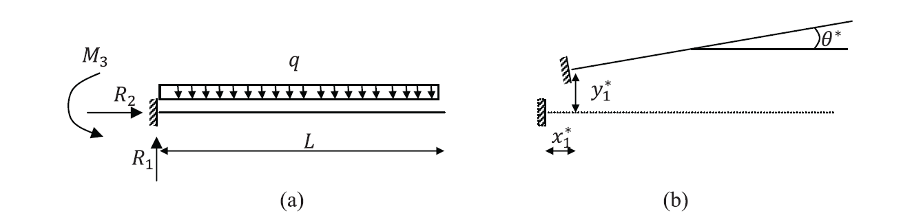
ExVW4 — Example 4. Virtual Work Principle in an Euler Bernoulli Cantilever Beam. (a) Geometry and Loading, (b) Rigid body displacement field.

SOLUTION:

There are three equilibrium equations which can be used to find the three unknown reactions:

$\sum F_{X_1}=R_2 = 0\qquad \sum F_{X_2}=R_1-qL = 0 \qquad \sum M_{@X_1=0}=\frac{qL^2}{2}-M_3=0$

Therefore, the three unknown reactions are:

$R_1=qL \qquad R_2=0 \qquad M_3=\frac{qL^2}{2}$

$y^*=y_1^*+X_1\sin{\theta^*}$

The statement of virtual work of the system is:

$R_1 y_1^* + R_2x_1^*+M_3\theta^*-\int_0^L\! qy^*\,\mathrm{d}X_1=0$

After substituting for $y^*$ and integrating, the above equation can be rearranged to have the following form:

$R_1y_1^* + R_2x_1^*+M_3\theta^*-qy_1^*L-\frac{qL^2}{2}\sin{\theta^*}=0$

Notice that the displacement field is chosen small enough such that $\theta^*=\sin{\theta^*}=\tan{\theta^*}$ . The above equation can then be rearranged to have the following form:

$(R_1-qL)y_1^* + \left(M_3-\frac{qL^2}{2}\right)\theta^*-R_2x_1^*=0$

Since the virtual displacement field is arbitrary and the statement applies for any choices of the variables $y_1^*$ , $x_1^*$ , and $\theta^*$ , then, their coefficients are equal to zero. Therefore, the three equations of equilibrium are retrieved:

$(R_1-qL)= 0\qquad M_3-\frac{qL^2}{2} = 0 \qquad R_2=0$

Therefore, the same reactions are obtained. Note that the chosen virtual displacement field guarantees that the associated internal virtual work is equal to zero.

Example 5: Application 2 of the Principle of Virtual Work

Use the principle of virtual work to find the displacement at the free end of the shown cantilever beam. Assume EI is constant and ignore the shearing force and normal force deformations.

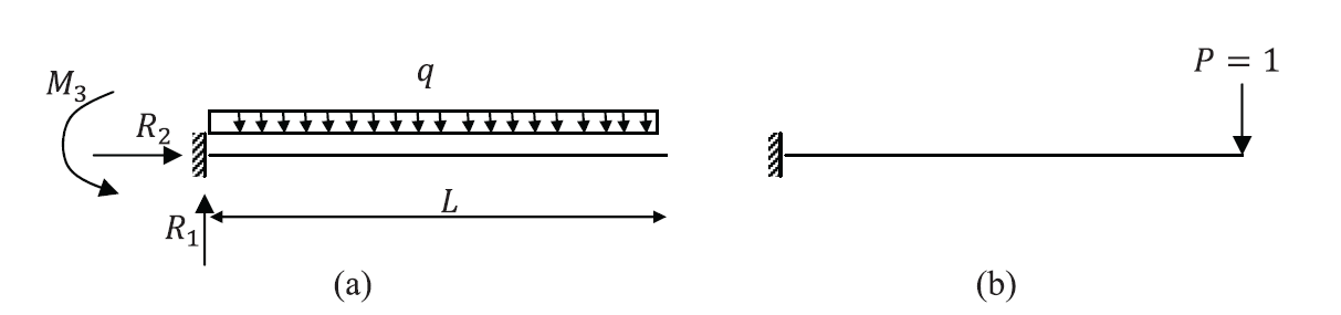
ExVW5 — Example 5. Virtual Work Principle to find the displacement in a statically determinate Euler Bernoulli Cantilever Beam. (a) Geometry and Loading, (b) Unit load.

SOLUTION:

The bending moment of the structure with the original load (distributed load) is given by the equation:

$M_0=-\frac{qL^2}{2}+qLX_1-\frac{qX_1^2}{2}$

After removing the loads from the structure and applying a unit load at the point of interest, the bending moment equation for the structure with the unit load $P=1$ is given by the equation:

$m_1=-PL + PX_1=X_1-L$

Applying the statement of virtual work as described above for this application:

$\int_0^L \! \frac{M_0m_1}{EI}\,\mathrm{d}X_1=1\times \Delta^*$

Therefore:

$\Delta ^*=\int_0^L \! \left(-\frac{qL^2}{2}+qLX_1-\frac{qX_1^2}{2}\right)\frac{(X_1-L)}{EI}\,\mathrm{d}X_1=\frac{qL^4}{8EI}$

Example 6: Application 3 of the principle of Virtual Work

Use the principle of virtual work to find an approximate cubic polynomial displacement solution for the shown beam. Compare with the exact solution for $\frac{P}{EI}=1$ unit and $L=1$ unit where $E, L$ and $I$ are the Young’s modulus, beam’s length, and moment of inertia respectively. Ignore Poisson’s ratio.

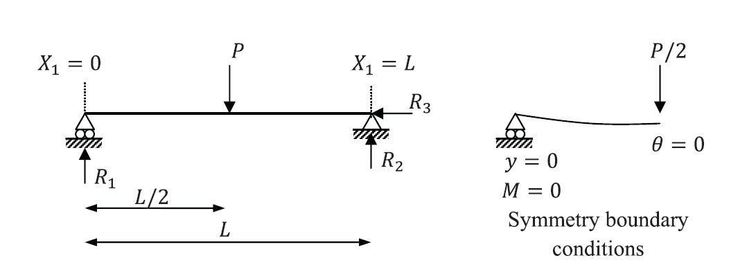
ExVW61 — Example 6. Geometry, loading and symmetry boundary conditions for an Euler Bernoulli beam.

SOLUTION:

First, we will find the exact displacement shape by solving the differential equation of equilibrium. Because of symmetry, we are going to solve the equation for only half the beam with the boundary conditions shown in the figure.

$EI\frac{\mathrm{d^4}y}{\mathrm{d}X_1^4}=q=0\Rightarrow EIy=\frac{C_1X_1^3}{6}+\frac{C_2X_1^2}{2}+C_3X_1+C_4$

The constants $C_1, C_2, C_3$ , and $C_4$ are integration constants and can be obtained from the four boundary conditions:

$\begin{split} @X_1=0:y=0\\ @X_1=0:M=EI\frac{\mathrm{d}^2y}{\mathrm{d}X_1^2}=0\\ @X_1=\frac{L}{2}:V=EI\frac{\mathrm{d}^3y}{\mathrm{d}X_1^3}=\frac{P}{2}\\ @X_1=\frac{L}{2}:\theta=\frac{\mathrm{d}y}{\mathrm{d}X_1}=0 \end{split}$

Therefore, the displacement function $y$ for $0\leq X_1 \leq \frac{L}{2}$ is given by:

$y=\frac{PX_1}{48EI}\left(-3L^2+4X_1^2\right)$

The displacement function for $\frac{L}{2}\leq X_1 \leq L$ can be obtained by replacing $X_1$ with $L-X_1$ in $y$ and thus the final displacement shape has the form:

$y=\begin{cases}\frac{PX_1}{48EI}\left(-3L^2+4X_1^2\right) & 0\leq X_1\leq \frac{L}{2}\\ \frac{P(L-X_1)}{48EI}\left(L^2-8X_1L+4X_1^2\right) & \frac{L}{2}\leq X_1\leq L \end{cases}$

The following are two important observations about the exact solution:

The exact solution is a polynomial of the third degree for each half.

We wish now to find an approximate solution for the displacement. We will force the solution however, to be continuous and differentiable at $X_1=\frac{L}{2}$ by assuming that the approximate solution is a cubic function applied from the whole length of the beam:

$y_{approx}=a_0+a_1X_1+a_2X_1^2+a_3X_1^3$

The first step in finding the appropriate coefficients $a_0, a_1, a_2$ , and $a_3$ is to ensure that this approximate solution satisfies the boundary conditions of displacement and rotation if any. Therefore we need to ensure:

$\begin{split} @X_1=0:y_{approx}=0\\ @X_1=L:y_{approx}=0 \end{split}$

Therefore,

$a_0=0\qquad a_1=-a_2L-a_3L^2$

Thus, the approximate displacement shape that would satisfy the boundary conditions has the form:

$y_{approx}=a_2X_1(X_1-L)+a_3X_1(X_1^2-L^2)$

The associated bending moment diagram in this case has the following form:

$M=EI\frac{\mathrm{d}^2y_{approx}}{\mathrm{d}X_1^2}=EI(2a_2+6a_3X_1)$

In order to apply the principle of virtual work, a virtual displacement needs to be assumed. Since the principle of virtual work applies for any assume virtual displacement, the most general virtual displacement field within the space of possible functions will be assumed. Since we restricted the solutions to be quadratic functions satisfying the boundary conditions, the most general virtual displacement has the form:

$y^*=a_2^*X_1(X_1-L)+a_3^*X_1(X_1^2-L^2)$

and the associated second derivative has the form:

$\frac{\mathrm{d}^2y^*}{\mathrm{d}X_1^2}=2a_2^*+6a_3^*X_1$

The internal virtual work can be calculated as follows:

$\begin{split} IVW & =\int_0^L \! EI\frac{\mathrm{d}^2y_{approx}}{\mathrm{d}X_1^2}\frac{\mathrm{d}^2y^*}{\mathrm{d}X_1^2}\,\mathrm{d}X_1=\int_0^L \! EI(2a_2+6a_3X_1)(2a_2^*+6a_3^*X_1)\,\mathrm{d}X_1\\ & =EI (4a_2La_2^* + 6a_3L^2 a_2^*+6a_2L^2a_3^*+12a_3L^3a_3^*)\\ & = EI(4a_2L+6a_3L^2)a_2^* + EI(6a_2L^2+12a_3L^3)a_3^* \end{split}$

On the other hand, the external virtual work has only one component due to the virtual work done by the force $P$ as the virtual displacement at the reactions is equal to zero:

$EVW=-Py^*|_{X_1=\frac{L}{2}}=-P\left(-\frac{a_2^*L^2}{4}-\frac{3a_3^*L^3}{8}\right)$

Since the principle of virtual applies to any choice for $a_2^*$ and $a_3^*$ , their multipliers on both sides of the equation of virtual work have to be equal. Therefore, we get the following two equations:

$4a_2L+6a_3L^2=\frac{PL^2}{4EI}\qquad 6a_2L^2+12a_3L^3=\frac{3PL^3}{8EI}$

Solving the above two equations yields:

$a_2=\frac{PL}{16EI}\qquad a_3=0$

Therefore, the best approximate solution that satisfies the virtual work principle is;

$y_{approx}=\frac{PL}{16EI}X_1(X_1-L)$

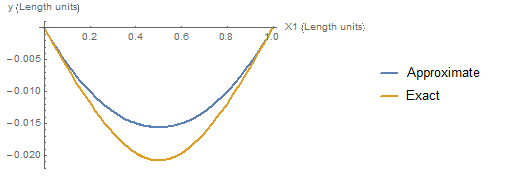
The approximate solution can be compared with the exact solution when $\frac{P}{EI}=L=1$ units. The plot of $y$ versus $X_1$ shows that the approximate solution under-predicts the displacement of the structure. In other words, the approximate solution gives a stiffer structure compared to the exact solution.

View Mathematica Code

Clear[y, P, X1, EI, L, yexact];
(*Exact solution*)
s = DSolve[{y''''[X1] == 0, y[0] == 0, y''[0] == 0, y'[L/2] == 0, 
    y'''[L/2] == P/2/EI}, y[X1], X1];
y1 = FullSimplify[y[X1] /. s[[1]]];
y2 = FullSimplify[y1 /. X1 -> L - X1];
yexact = Piecewise[{{y1, 0 <= X1 < L/2}, {y2, L/2 <= X1 <= L}}];
(*Approximate solution*)
yapprox = a2*X1*(X1 - L) + a3*X1*(X1^2 - L^2);
ystar = yapprox /. {a2 -> a2s, a3 -> a3s};
EVW = -P*ystar /. X1 -> L/2;
IVW = Integrate[EI*D[yapprox, {X1, 2}]*D[ystar, {X1, 2}], {X1, 0, L}];
Eq1 = Coefficient[IVW, a2s] - Coefficient[EVW, a2s];
Eq2 = Coefficient[IVW, a3s] - Coefficient[EVW, a3s];
s = Solve[{Eq1 == 0, Eq2 == 0}, {a2, a3}];
yapprox = yapprox /. s[[1]];
yp = yapprox /. {P -> 1, EI -> 1, L -> 1};
yexactp = yexact /. {P -> 1, EI -> 1, L -> 1};
Plot[{yp, yexactp}, {X1, 0, 1}, 
 PlotLegends -> {"Approximate", "Exact"}, 
 AxesLabel -> {"X1 (Length units)", "y (Length units)"}]

View Python Code

from sympy import Function,dsolve,diff,integrate,Poly,solve,simplify
import numpy as np
import matplotlib.pyplot as plt
y = Function("y")
x,EI,L,P = sp.symbols("x EI L P")
a2,a3,a2s,a3s = sp.symbols("a_2 a_3 a_2s a_3s")
y1 = y(x).subs({x:0})
th2 = y(x).diff(x).subs(x,L/2)
M1 = y(x).diff(x,2).subs(x,0)
V2 = y(x).diff(x,3).subs(x,L/2)
s = dsolve(y(x).diff(x,4),y(x),ics={y1:0,th2:0,M1:0,V2:P/2/EI})
y1 = s.rhs
y2 = simplify(y1.subs({x:L-x}))
yapprox = a2*x*(x-L)+a3*x*(x**2-L**2)
ystar = yapprox.subs({a2:a2s,a3:a3s})
EVW = (-P*ystar).subs({x:L/2}).expand()
IVW = integrate(EI*diff(yapprox,x,x)*diff(ystar,x,x),(x,0,L)).expand()
Eq1 = IVW.coeff(a2s)-EVW.coeff(a2s)
Eq2 = IVW.coeff(a3s)-EVW.coeff(a3s)
s = solve({Eq1,Eq2},{a2,a3})
yapprox = yapprox.subs({a2:s[a2],a3:s[a3]})
y1exactp = y1.subs({L:1,EI:1,P:1})
y2exactp = y2.subs({L:1,EI:1,P:1})
yp = yapprox.subs({L:1,EI:1,P:1})
xL = xrange = np.arange(0,1.01,0.01)
Y1 = []
Y2 = []
for i in range(len(xL)):
    Y1.append(yp.subs({x:xL[i]}))
    #piecewise for exact : y1 when 0<=x<L/2, y2 when L/2=<x<L
    if i<(len(xL)/2):
        Y2.append(y1exactp.subs({x:xL[i]}))
    else:
        Y2.append(y2exactp.subs({x:xL[i]}))
fig, ax = plt.subplots()
plt.xlabel("x(length units)")
plt.ylabel("y(length units)")
ax.plot(xL, Y1, label="Approx")
ax.plot(xL, Y2, label="Exact")
ax.legend()
ax.grid(True, which='both')
ax.axhline(y = 0, color = 'k')
ax.axvline(x = 0, color = 'k')

Video

Problems

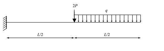
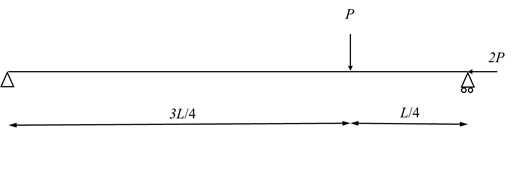
Use the principle of virtual work to find the reactions for the following statically determinate structures.
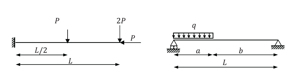
Use the principle of virtual work to find the reactions for the following statically determinate structures.
The shown beams have Young’s modulus $E$ and moment of inertia $I$ . Verify that the virtual work principle applies assuming a virtual displacement field $y^*=aX_1(X_1-L)$ where $a>0$ .
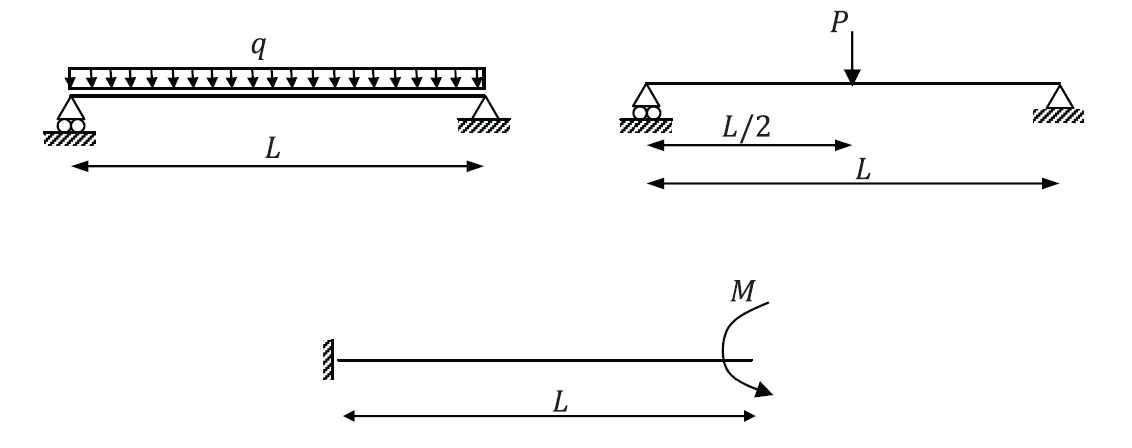
Repeat the previous question assuming a virtual displacement field $y^*=aX_1^2$ where $a>0$ .
The Cauchy stress distribution in the shown plate is given by:
$\sigma=\left(\begin{matrix}x_1&3&0\\3&0&0\\0&0&0\end{matrix}\right)KN/m^2$
where and are the coordinates inside the plate with units of m. Find the equilibrium body forces vector applied to the plate. Find the traction forces on the boundary edges , and of the plate. Verify the principle of virtual work in the following two cases:
- Assuming a virtual displacement field $u_1^*=ax_1, a>0$ .
- Assuming a virtual displacement field $u_2^*=bx_1, b>0$ .
The Cauchy stress distribution on the shown unit length cube is given by:
$\sigma=\left(\begin{matrix}x_1x_2&4&2\\4&x_1&0\\2&0&x_3\end{matrix}\right)KN/m^2$
where , and are the coordinates inside the cube with units of .
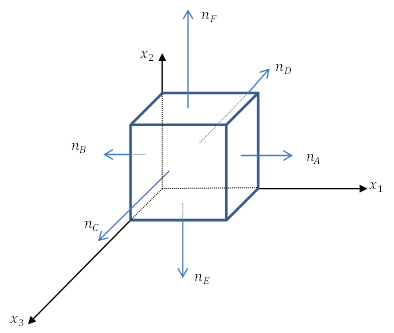
1. Find the equilibrium body forces vector applied on the cube.
2. Find the traction vectors on the boundary faces $A, B, C, D, E$ , and $F$ of the cube.
3. Verify the principle of virtual work for the following virtual displacement field
  $u^*=\left(\begin{matrix}ax_1\\bx_2\\cx_3\end{matrix}\right)$
  where $a,b$ , and $c$ are positive real numbers.
Use the principle of virtual work to find approximate linear, quadratic, cubic, and quartic polynomial displacement solutions for a simply supported beam with length $L$ , Young’s modulus $E$ , moment of inertia $I$ , and a distributed load $q$ . Compare the approximate solutions with the exact solution for $q=1$ units, $EI=1$ units, and $L=2$ units. Ignore Poisson’s ratio.