Engineering at Alberta Courses » One Dimensional Quadratic Elements

FEA in One Dimension: One Dimensional Quadratic Elements

One Dimensional Quadratic Elements

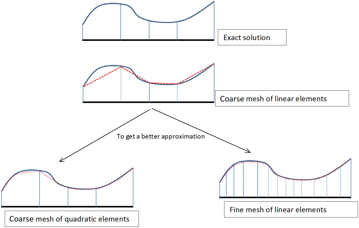
In the previous section, the domain of a one-dimensional problem was discretized using piecewise linear functions. Another approximation is the C0 piecewise quadratic interpolation functions, where on each element, the displacement is quadratic. If one wishes to obtain better accuracy, either a finer mesh of linear elements is to be used, or quadratic elements are to be used instead of the linear elements (Figure 5).

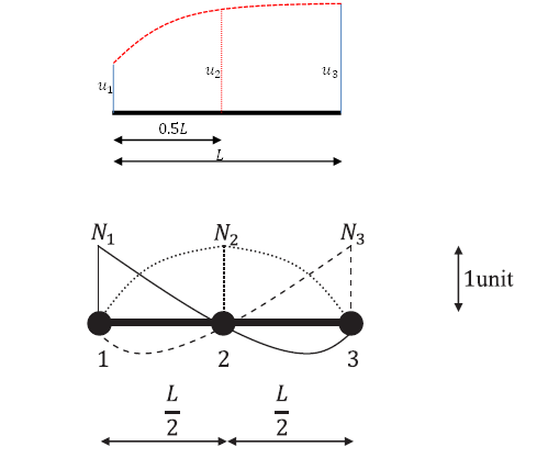
Figure 5. Linear vs. quadratic one dimensional elements

To define a quadratic one dimensional element, an additional inner node is introduced. Similar to the linear elements, the displacement function is continuous across nodes but not differentiable at the boundaries between elements. In general, the quadratic form of the displacement is:

$u = a_0 + a_1X_1 + a_2 X_1^2$

Figure 6 shows the displacement function of a quadratic element with three nodes. An alternative form of the displacement is:

$u = u_1N_1 + u_2N_2 + u_3N_3$

where $u_1$ , $u_2$ , and $u_3$ are the displacements of the nodes 1, 2, and 3, while $N_1$ , and $N_2$ , and $N_3$ are the shape functions associated with these nodes (Figure 6). $a_0$ , $a_1$ , and $a_2$ are the generalized degrees of freedom of the element while $u_1$ , $u_2$ , and $u_3$ are the nodal degrees of freedom. To find the shape functions $N_1$ , $N_2$ , and $N_3$ , the following three equations are solved:

$@X_1 = 0: u = u_1 \Rightarrow a_0 = u_1$

$@X_1 = \frac{L}{2}: u = u_2 \Rightarrow a_0 + a_1\frac{L}{2} + a_2\frac{L^2}{4} = u_2$

$@X_1 = L: u = u_3 \Rightarrow a_0 + a_1L + a_2L^2 = u_3$

Therefore,

$a_0 = u_1$

$a_1 = -\frac{3u_1-4u_2+u_3}{L}$

$a_2 = \frac{2(u_1 -2u_2 + u_3)}{L^2}$

Therefore, the displacement function in terms of the nodal degrees of freedom has the form:

$u = u_1 - \frac{3u_1 -4u_2 + u_3}{L} X_1 + \frac{2(u_1 -2u_2+u_3)}{L^2} X_1^2$

Rearranging:

$u = u_1 \Big(\frac{(L-2X_1)(L-X_1)}{L^2} \Big) + u_2 \Big(\frac{4(L-X_1)X_1}{L^2} \Big) + u_3 \Big(\frac{-(L-2X_1)X_1}{L^2} \Big)$

Therefore, the shape functions are:

$N_1 = \frac{(L-2X_1)(L-X_1)}{L^2}$

$N_2 = \frac{4(L-X_1)X_1}{L^2}$

$N_3 = \frac{-(L-2X_1)x_1}{L^2}$

Figure 6. One dimensional quadratic element displacement function and shape functions

It can be checked that the sum of the shape functions is always equal to 1, which allows for the rigid-body motion or constant displacement of an element to be modelled (Why?). The local stiffness matrix and the local nodal forces vectors can be established similar to the previous section. First, the following matrices are defined:

$N = \hspace{1mm} < \hspace{2mm} N_1 \hspace{2mm} N_2 \hspace{2mm} N_3 \hspace{2mm} > \hspace{1mm}$

$B = \hspace{1mm} < \hspace{2mm} \frac{dN_1}{dX_1} \hspace{2mm} \frac{dN_2}{dX_1} \hspace{2mm} \frac{dN_3}{dX_1} \hspace{2mm} > \hspace{1mm}$

$u_e = \begin{pmatrix} u_1 \\ u_2 \\ u_3 \\ \end{pmatrix}$

then the displacement $u$ , $\varepsilon_{11}$ , and $\sigma_{11}$ can be written in terms of the nodal degrees of freedom vector $u_e$ as follows:

$u = Nu_e$

$\varepsilon_{11} = Bu_e$

$\sigma_{11} = EBu_e$

If $E$ is Young’s modulus and $A$ is the cross sectional area of the element, then the local stiffness matrix of the element is a $3\times 3$ matrix and has the form:

$K^e = \int_{0}^L EAB^TBdX_1$

If $E$ and $A$ are constant, then $K^e$ has the form:

$K^e = \frac{EA}{3L} \begin{pmatrix} 7 & -8 & 1 \\ -8 & 16 & -8 \\ 1 & -8 & 7 \\ \end{pmatrix}$

The nodal forces vector is a 3 dimensional vector and has the form:

$f^e = \int_0^L pN^T dX_1$

where $p$ is the distributed load per unit length acting on the element. If $p$ is constant, then the nodal forces vector have the form:

$f^e = pL \begin{pmatrix} \frac{1}{6} \\ \frac{2}{3} \\ \frac{1}{6} \\ \end{pmatrix}$

View Mathematica Code

u = a0 + a1*X1 + a2*X1^2;
Eq1 = u /. X1 -> 0;
Eq2 = u /. X1 -> L/2;
Eq3 = u /. X1 -> L;
a = Solve[{Eq1 == u1, Eq2 == u2, Eq3 == u3}, {a0, a1, a2}]
u = u /. a[[1]]
N1 = FullSimplify[Coefficient[u, u1]]
N2 = FullSimplify[Coefficient[u, u2]]
N3 = FullSimplify[Coefficient[u, u3]]
B = {{D[N1, X1], D[N2, X1], D[N3, X1]}};
B // MatrixForm
Transpose[B] // MatrixForm
K = EA*Integrate[Transpose[B].B, {X1, 0, L}];
K // MatrixForm
Nn = {{N1, N2, N3}};
fe = Integrate[p*Transpose[Nn], {X1, 0, L}];
fe // MatrixForm

View Python Code

import sympy as sp
from sympy import solve,Matrix,diff,integrate
a0,a1,a2,x,L,EA,p = sp.symbols("a_0 a_1 a_2 x L EA p")
u1,u2,u3 = sp.symbols("u_1 u_2 u_3")
u = a0+a1*x+a2*x**2
display("Quadratic Form of Displacement:")
display("u =", u)
eq1 = u.subs({x:0})
eq2 = u.subs({x:L/2})
eq3 = u.subs({x:L})
s = solve((eq1-u1,eq2-u2,eq3-u3),a0,a1,a2)
display("Solve")
display("a_0 =",s[a0],"a_1 =",s[a1],"a_2 =",s[a2])
u = u.subs(s).expand()
display("Rearranging")
display("u =",u)
N1 = u.coeff(u1)
N2 = u.coeff(u2)
N3 = u.coeff(u3)
display("Shape Functions")
B = Matrix([[diff(N1,x),diff(N2,x),diff(N3,x)]])
display("B =",B.T)
K = EA*Matrix([[integrate(B[i]*B[j], (x,0,L)) for i in range(3)] for j in range(3)])
display("K^e =",K)
Nn = Matrix([[N1,N2,N3]]).T
display("N =",Nn)
fe = Matrix([p*integrate(Nn[i],(x,0,L))for i in range(3)])
display("Nodal Force Vector")
display("f^e =",fe)

Problems

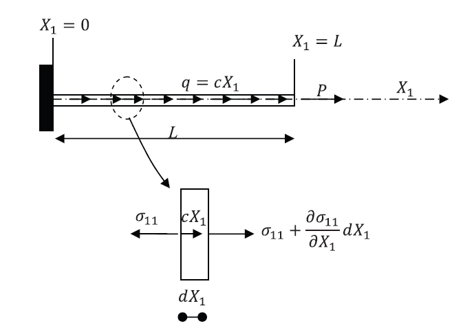
For a quadratic one dimensional element of length L, find the nodal forces vector if a distributed horizontal load of $p(X_1)=5+X_1/L$ (load per unit length) is applied on the element.
Using two quadratic one dimensional elements and the virtual work method, find the displacement of the nodes and the stress within each element of the following problem assuming $c=1$ , $E=1$ , $A=1$ , and $L=1$ units. Compare with the exact solution and the solution using four linear elements shown above.

Open Educational Resources

FEA in One Dimension: One Dimensional Quadratic Elements

One Dimensional Quadratic Elements

Problems

Leave a Reply Cancel reply