Strain Measures: Examples and Problems

Example 1:

Calculate the infinitesimal and Green strain matrices for the following position function:

Also, find the displacement function, the uniaxial small and Green strains along the direction of the vector .

Solution:

The displacement function is:

The small strain tensor is:

The Green strain tensor is:

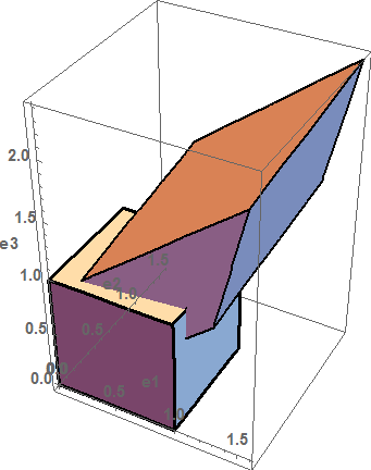
The deformation is very large as shown by applying this deformation to a unit cube (see figure below), so the strain measures are different.

The uniaxial small and Green strain along the vector can be obtained as follows:

View Mathematica Code

View Python Code

from sympy import *
import sympy as sp
sp.init_printing(use_latex="mathjax")
F = Matrix([[1.2,0.2,0.2],[0.2,1.3,0.1],[0.9,0.5,1]])
X1,X2,X3 = sp.symbols("X1 X2 X3")
x1,x2,x3 = sp.symbols("x1 x2 x3")
X = Matrix([X1,X2,X3])
x = Matrix([x1,x2,x3])
display("X =",X)
display("x =",x)
display("x = F.X =",F*x)
x = F*X
u = x-X
display("u = x-X =",u)
gradu = Matrix([[diff(i,j) for j in X] for i in u])
display("\u2207u =",gradu)
small_strain = (gradu+gradu.T)/2
display("\u03B5_small =",small_strain)
green_strain = (gradu+gradu.T+gradu.T*gradu)/2
display("\u03B5_Green =",green_strain)
v = Matrix([1,1,1])
n = v/v.norm()
display("small strain along u", n.dot(small_strain*n))
display("Green strain along u", n.dot(green_strain*n))

Example 2:

A cube of unit dimensions undergoes a rigid body rotation in of , then , and then around the basis vectors and respectively. Use Mathematica to visualize the box. Compare the two strain measures and .

SOLUTION:

The deformation gradient is given by:

Note that is on the right since it is applied first.
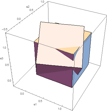
The Green strain is identically zero while the small strain tensor predicts the following strains:

View Mathematica Code

View Python Code

from sympy import *
import sympy as sp
theta = sp.symbols("\u03B8")
X1,X2,X3=sp.symbols("X1 X2 X3")
x1,x2,x3=sp.symbols("x1 x2 x3")
Qx = Matrix([[1, 0, 0], 
              [0, sp.cos(theta),-sp.sin(theta)], 
              [0, sp.sin(theta),sp.cos(theta)]])
# y rotation matrix
Qy = Matrix([[sp.cos(theta), 0, sp.sin(theta)], 
              [0, 1, 0], 
              [-sp.sin(theta), 0, sp.cos(theta)]])
# z rotation matrix
Qz = Matrix([[sp.cos(theta), -sp.sin(theta), 0],
              [sp.sin(theta), sp.cos(theta), 0], 
              [0, 0, 1]])
Qx = Qx.subs({theta:30*sp.pi/180})
Qy = Qy.subs({theta:20*sp.pi/180})
Qz = Qz.subs({theta:20*sp.pi/180})
F = Qx*Qy*Qz
display("F =",F)
F = simplify(F).evalf()
display("F =",F)
X=Matrix([X1,X2,X3])
x=Matrix([x1,x2,x3])
display("X =",X)
display("x =",x)
display("x =F.X =",F*x)
x = F*X
u = x-X
display("u = x-X =",u)
gradu = Matrix([[diff(i,j) for j in X] for i in u])
display("\u2207u =",gradu)
small_strain = (gradu+gradu.T)/2
display("\u03B5_small =",small_strain)
green_strain = (gradu+gradu.T+gradu.T*gradu)/2
display("\u03B5_Green =",green_strain)

Example 3:

A cube of unit length undergoes a simple shearing motion of an angle in the direction of and perpendicular to . Find the infinitesimal and Green strain measures that describe this motion. Comment on the difference between the two strain measures.

SOLUTION:

The position function is given by:

The deformation gradient is given by:

The small strain and Green strain tensors are given by:

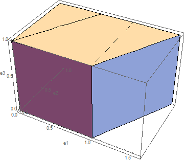
Both measures predict the same shear strains. For small deformations, both measures predict zero normal strains. As the increases, the vertical lines start developing large axial strains which the can predict while cannot. The undeformed and deformed shapes of the cube are shown below for .

View Mathematica Code

View Python Code

from sympy import *
import sympy as sp
sp.init_printing(use_latex="mathjax")
X1, X2, X3 = sp.symbols("X_1 X_2 X_3")
theta = sp.symbols("\u03B8")
X = Matrix([X1, X2, X3])
F = Matrix([[1,tan(theta),0],[0,1,0],[0,0,1]])
display("deformation gradient:")
display("F =",F)
x = F*X
display("position function:")
display("x =",x)
u = x-X
display("u = x-X =",u)
gradu = Matrix([[diff(i,j) for j in X] for i in u])
display("\u2207u =",gradu)
small_strain = (gradu+gradu.T)/2
display("\u03B5_small =",small_strain)
green_strain = (gradu+gradu.T+gradu.T*gradu)/2
display("\u03B5_Green =",green_strain)

Example 4:

The following small strain matrix represents a two dimensional state of strain

Find the principal strains and their directions. If a coordinate system is aligned with the principal directions, find the components of the strain matrix in this new coordinate system.

SOLUTION:

The principal strains and and their directions , and be obtained using Mathematica by finding the eigenvalues and eigenvectors of . The following are the eiganvalues:

The following are the normalized eigenvectors.

The transformation matrix between the original coordinate system and the new coordinate system is:

The strain matrix in the new coordinate system has the form:

View Mathematica Code

View Python Code

from sympy import *
import sympy as sp
sp.init_printing(use_latex="mathjax")
small_strain = Matrix([[0.01, 0.012],[0.012, 0]])
display("\u03B5_small =",small_strain) 
# eigenvalues
eigensystem = small_strain.eigenvects()
display("eigensystem", eigensystem)
eigenvalues = [i[0] for i in eigensystem]
eigenvectors = [i[2][0].T for i in eigensystem]
neigenvectors = [i/i.norm() for i in eigenvectors]
display("eigenvalues (principal strains) =",eigenvalues)
display("eigenvectors (principal directions) =",eigenvectors)
display("Normalized eigenvectors (principal directions) =",neigenvectors)
#The function Matrix ensures the list is a sympy matrix
Q = Matrix(neigenvectors)
display("Diagonalized matrix = Q.M.Q^T",Q*small_strain*Q.T)
display("Diagonalized matrix = Q.M.Q^T",N(Q*small_strain*Q.T,chop=True))

Example 5:

A state of uniform small strain is described by the following small strain matrix:

Determine the following:

• The longitudinal strain along the direction of the vector .
• The change in the cosines of the angles between the vectors and and comment on whether the angle between the vectors decreased or increased after deformation.
• The shear strains of planes parallel to the vector and perpendicular to the vector .

SOLUTION:

The strains along can be calculated as follows:

The change in the cosines of the angles between the vectors and can be calculated as follows:

The angle between the vectors and before deformation can be calculated using the dot product:

Therefore, the angle after deformation between the vectors is larger because:

Since the vectors and are perpendicular, the shear strains of planes parallel to the vector and perpendicular to the vector can be obtained as follows:

View Mathematica Code

View Python Code

import sympy as sp
from sympy import *
sp.init_printing(use_latex="mathjax")
small_strain = Matrix([[-0.01, 0.002, -0.023],[0.002, 0.05, 0],[-0.023, 0, 0.02]])
display("\u03B5_small =",small_strain)
# part 1
display("part 1")
dX = Matrix([1,2,1])
display("dX =",dX)
display("norm of dX =",dX.norm())
ndX = dX/dX.norm()
display("small strain along dX =",ndX.dot(small_strain*ndX))
# part 2
display("part 2")
dX = Matrix([1,0,1])
dY = Matrix([1,1,1])
display("dX =",dX)
display("dY =",dY)
ndX = dX/dX.norm()
ndY = dY/dY.norm()
small_strain_along = ndX.dot(small_strain*ndY)
display("1/2 change of cos of angle between dX and dY =",small_strain_along.evalf())
phi = acos(ndX.dot(ndY)).evalf()
display("\u03A6 =",phi,"degrees", deg(phi).evalf())
theta = acos(small_strain_along*2 + cos(phi))
display("\u03B8 =",theta,"degrees", deg(theta).evalf())
# part 3
display("part 3")
dX = Matrix([-1,1,0])
dY = Matrix([1,1,0])
display("dX =",dX)
display("dY =",dY)
ndX = dX/dX.norm()
ndY = dY/dY.norm()
display("shear strain =",ndX.dot(small_strain*ndY).evalf())

Example 6:

The longitudinal engineering strains on the surface of a test specimen were measured using a strain gauge rosette to be 0.005, 0.002 and –0.001 along the three directions: , , and respectively, where . If the material is assumed to be in a small strain state, find the principal strains and their directions on the surface of the test specimen.

SOLUTION:

The state of strain on the surface of the material can be represented by the symmetric small strain matrix:

Since the longitudinal strain is known along three directions, three equations can be written to find the three unknown components of the strain matrix as follows:

The norm of each of a, b, and c is 1. Therefore, the three equations are:

Solving the above three equations yields:

The principal strains and their directions are the eigenvalues and eigenvectors of the small strain matrix. The principal strains are:

The principal directions are:

View Mathematica Code

View Python Code

from sympy import *
import sympy as sp
sp.init_printing(use_latex="mathjax")
E11, E12, E22 = sp.symbols("\u03B5_{11} \u03B5_{12} \u03B5_{22}")
E_s = sp.symbols("\u03B5_{small}=")
E_small = Matrix([[E11, E12],[E12, E22]])
display(E_s,E_small)
theta = sp.symbols("\u03B8")
a = Matrix([sp.cos(theta), sp.sin(theta)])
b = Matrix([0,1])
c = Matrix([-sp.cos(theta), sp.sin(theta)])
a, c = a.subs({theta:30*sp.pi/180}), c.subs({theta:30*sp.pi/180})
display("a =",a)
display("b =",b)
display("c =",c)
strain = Matrix([Rational('5/1000'), Rational('2/1000'),Rational('-1/1000')])
eq1 = simplify(a.dot(E_small*a)) - strain[0]
eq2 = simplify(b.dot(E_small*b)) - strain[1]
eq3 = simplify(c.dot(E_small*c)) - strain[2]
display("Systems of equations:")
display(eq1)
display(eq2)
display(eq3)
sol = solve([eq1, eq2, eq3],[E11, E12, E22])
E_small = E_small.subs({E11:sol[E11],E12:sol[E12],E22:sol[E22]})
display(E_s,E_small)
E_small = N(E_small)
display(E_s,E_small)
eigensystem = E_small.eigenvects()
display("eigensystem", eigensystem)
eigenvalues=[i[0] for i in eigensystem]
eigenvectors=[i[2][0].T for i in eigensystem]
neigenvectors=[i/i.norm() for i in eigenvectors]
display("eigenvalues (principal strains) =",eigenvalues)
display("eigenvectors (principal directions) =",eigenvectors)
display("Normalized eigenvectors (principal directions) =",neigenvectors)

Example 7:

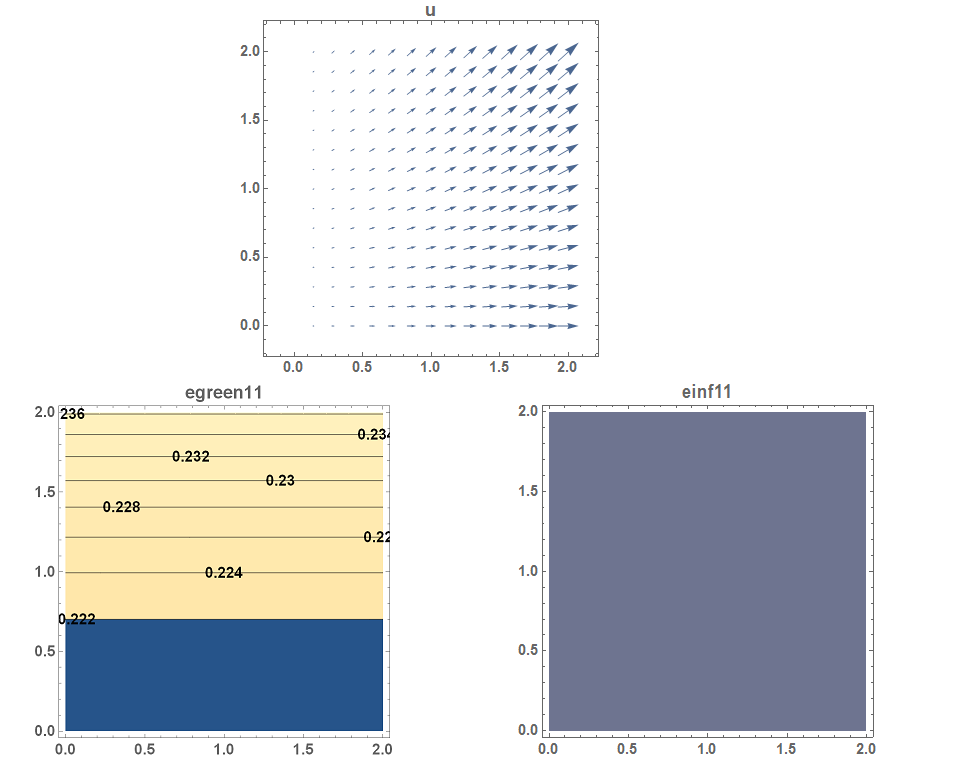
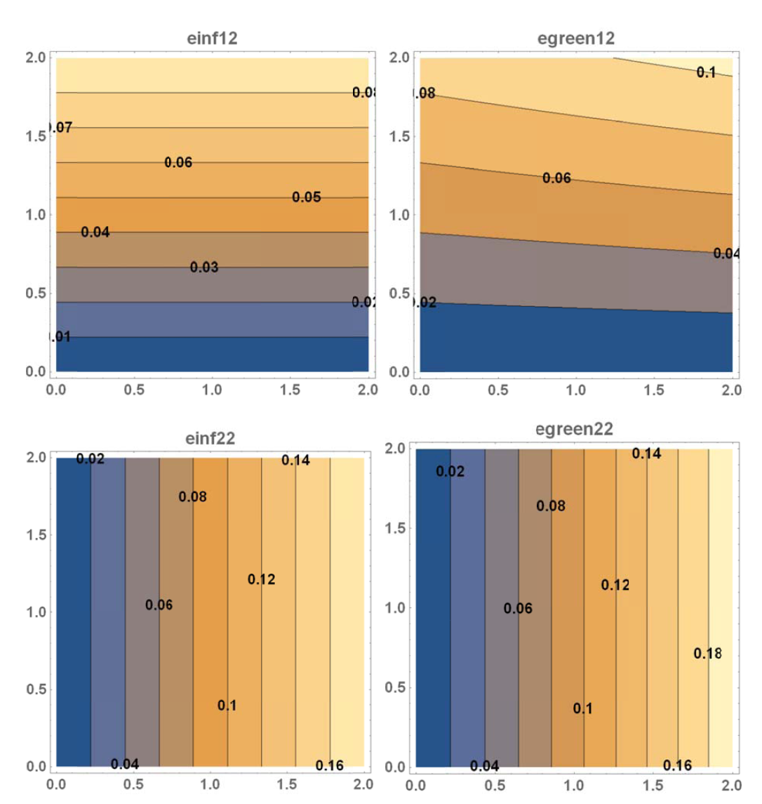
In the above examples, the deformation was described by a uniform strain matrix (i.e., a strain matrix that is not function in position). In this example, a nonuniform strain, i.e., the strain matrix is function of position is explored. Assume that the two dimensional displacement function of a 2units by 2units plate has the following form:

• Find the deformed configuration function .
• Find and .
• Draw the vector plot of the displacement function on the plate.
• Draw the contour plots of , , , and on the plate.

SOLUTION:

The position function of the deformed configuration is given by:

The deformation gradient is given by:

The displacement gradient is given by:

Therefore, the small strain matrix is given by:

The Green strain matrix is given by:

The required plots are shown below.

View Mathematica Code

Clear[x1, x2, X1, X2]
X = {X1, X2};
u = {0.2 X1, 0.09 X2*X1};
x = u + X;
Gradu = Table[D[u[[i]], X[[j]]], {i, 1, 2}, {j, 1, 2}]
einfinitesimal = 1/2*(Gradu + Transpose[Gradu]);
egreen = 1/2*(Gradu + Transpose[Gradu] + Transpose[Gradu] . Gradu);
einfinitesimal // MatrixForm
FullSimplify[egreen] // MatrixForm
u
VectorPlot[u, {X1, 0, 2}, {X2, 0, 2}, 
 BaseStyle -> Directive[Bold, 15], AspectRatio -> Automatic, 
 PlotLabel -> "u"]
ContourPlot[einfinitesimal[[1, 1]], {X1, 0, 2}, {X2, 0, 2}, 
 BaseStyle -> Directive[Bold, 15], AspectRatio -> Automatic, 
 ContourLabels -> All, PlotLabel -> "einf11"]
ContourPlot[egreen[[1, 1]], {X1, 0, 2}, {X2, 0, 2}, 
 BaseStyle -> Directive[Bold, 15], AspectRatio -> Automatic, 
 ContourLabels -> All, PlotLabel -> "egreen11"]
ContourPlot[einfinitesimal[[1, 2]], {X1, 0, 2}, {X2, 0, 2}, 
 BaseStyle -> Directive[Bold, 15], AspectRatio -> Automatic, 
 ContourLabels -> All, PlotLabel -> "einf12"]
ContourPlot[egreen[[1, 2]], {X1, 0, 2}, {X2, 0, 2}, 
 BaseStyle -> Directive[Bold, 15], AspectRatio -> Automatic, 
 ContourLabels -> All, PlotLabel -> "egreen12"]
ContourPlot[einfinitesimal[[2, 2]], {X1, 0, 2}, {X2, 0, 2}, 
 BaseStyle -> Directive[Bold, 15], AspectRatio -> Automatic, 
 ContourLabels -> All, PlotLabel -> "einf22"]
ContourPlot[egreen[[2, 2]], {X1, 0, 2}, {X2, 0, 2}, 
 BaseStyle -> Directive[Bold, 15], AspectRatio -> Automatic, 
 ContourLabels -> All, PlotLabel -> "egreen22"]
View Python Code

from sympy import *
import sympy as sp
from mpl_toolkits.mplot3d import Axes3D
import matplotlib.pyplot as plt
import numpy as np
sp.init_printing(use_latex="mathjax")
# calculation
X1, X2 = sp.symbols("X_1 X_2")
u = Matrix([0.2*X1, 0.09*X2*X1])
display("u =",u)
X = Matrix([X1, X2])
x = X + u
display("x =", x)
F = Matrix([[diff(xi,Xj) for Xj in X] for xi in x])
display("F =",F)
grad_u = F - eye(2)
display("\u2207u =",grad_u)
small_strain = (grad_u+grad_u.T)/2
display("small strain =",small_strain)
green_strain = (grad_u+grad_u.T+grad_u.T*grad_u)/2
display("green strain =",green_strain)
# plots

# vector plots
def plotVector(f, limits, title):
    fx, fy = [lambdify((X1,X2),fi) for fi in f]
    x1, xn, y1, yn = limits
    dx, dy = 10/100*(xn-x1),10/100*(yn-y1)
    xrange = np.arange(x1,xn,dx)
    yrange = np.arange(y1,yn,dy)
    X, Y = np.meshgrid(xrange, yrange)
    dxplot, dyplot = fx(X,Y), fy(X,Y)
    fig = plt.figure()
    ax = fig.add_subplot(111)
    ax.quiver(X, Y, dxplot, dyplot)
    plt.title(title)
# contour plots
def plotContour(f, limits, title):
    x1, xn, y1, yn = limits
    dx, dy = 10/100*(xn-x1),10/100*(yn - y1)
    xrange = np.arange(x1,x1+xn,dx)
    yrange = np.arange(y1,y1+yn,dy)
    X, Y = np.meshgrid(xrange, yrange)
    lx, ly = len(xrange), len(yrange)
    F = lambdify((X1,X2),f)
    # if F is constant, then generates array
    # if F generates array, doesn't change anything
    Z = F(X,Y)*np.ones(lx*ly).reshape(lx, ly)
    fig = plt.figure()
    ax = fig.add_subplot(111)
    cp = ax.contourf(X,Y,Z)
    fig.colorbar(cp)
    plt.title(title)
# vector plot of u
plotVector(u,[0,2,0,2],'u' )
# small strain plots
plotContour(small_strain[0,0],[0,2,0,2],'\u03B5_small (1,1)')
plotContour(small_strain[0,1],[0,2,0,2],'\u03B5_small (1,2)')
plotContour(small_strain[1,1],[0,2,0,2],'\u03B5_small (2,2)')
# green strain plots
plotContour(green_strain[0,0],[0,2,0,2],'\u03B5_Green (1,1)')
plotContour(green_strain[0,1],[0,2,0,2],'\u03B5_Green (1,2)')
plotContour(green_strain[1,1],[0,2,0,2],'\u03B5_Green (2,2)')

Problems:

1. Which of the following functions describing motion is/are not physically possible and why?
   • 
   • 
   • 
   • 
2. Calculate the limits of and for the following position functions to be physically possible:
   • .
   • .
   • .
3. Let a cube of unit length be represented by the set of vectors such that three of the cube’s sides are aligned with the three orthonormal basis set vectors , , and and one of the cube vertices lies on the origin of the coordinate system. Let be the deformed configuration such that is defined as :

      

   Find the following:
   • The displacement function .
   • The new position of the 8 vertices of the cube.
   • The deformed curves of the three edges of the cube that are aligned with the basis vectors , , and .
   • The infinitesimal strain matrix and the volumetric strain as a function of the position inside the cube.
   • The Green strain matrix as a function of the position inside the cube.
   • Evaluate the infinitesimal strain matrix at two of the eight cube vertices.
   • Evaluate the Green strain matrix at two of the eight cube vertices.
4. The reference and deformed configurations of an object exhibiting a two dimensional motion is shown in the figure below.

   

   Find the following: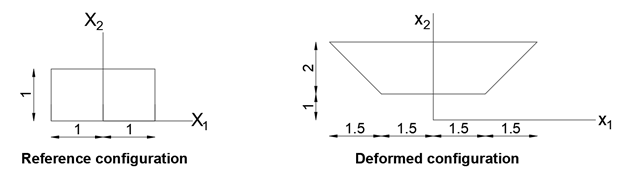
   • The two dimensional position function that can describe this shown motion.
   • The associated two dimensional displacement function. The associated small strain tensor.
   • The associated Green Lagrange strain tensor.
5. A cube undergoes a deformation such that the infinitesimal strain is described by the matrix:

      

   Find the following:
   • The principal strains and their directions.
   • The longitudinal strains along the direction of the vector:

        

   • The approximate change in the angles between the vectors dX and

        

   • The coordinate system transformation in which the strain matrix is diagonal. Express the strain matrix in the new coordinate system.
6. The longitudinal engineering strains on the surface of a test specimen were measured using a strain rosette to be 0.005, 0.002, and –0.001 along the three directions: , , and where is along the direction of the basis vector , is oriented anticlockwise from , and is oriented anticlockwise from . If the material is assumed to be in a small strain state, find the principal strains and their directions on the surface of the test specimen.
7. The longitudinal engineering strains on the surface of a test specimen were measured using a strain rosette to be 0.006, -0.001, and 0.002 along the three directions: , , and where a is along the direction of the basis vector , is oriented anticlockwise from , and is oriented anticlockwise from . If the material is assumed to be in a small strain state, find the principal strains and their directions on the surface of the test specimen.
8. The measured strains for the three axes of a strain gauge rosette are: , , and . If coincides with the basis vector while and coincide with vectors that are anticlockwise and respectively from . Find the components of the strain tensor.
9. Assume that a two dimensional rectangular plate with dimensions 5 units along the basis vector and 1 unit along the basis vector is situated such that the origin of the coordinate system is at the midpoint of the left side of the plate. If the displacement function of the plate is described by:

      

   find the following:
   • The position function .
   • The infinitesimal strain matrix as a function of the position.
   • The Green strain matrix as a function of the position.
   • Draw the vector plot of the displacement function.
   • Draw the contour plots of , , , and .
10. Repeat the previous question if the displacement function is given by:

       

11. The general equation for the coordinates of a point x on an ellipsoidal surface whose axes are oriented along the Cartesian coordinate system is:

       

    where , , and are the three semi-diameters of the ellipsoidal surface. When , the surface is a sphere with radius . Assuming that the motion of an object is described by the homogeneous deformation gradient such that the diagonal components of are the only non-zero components.
    • Show that a sphere of radius deforms into an ellipsoid surface.
    • Find the relationship between the semi-diameters of the ellipsoid and the components of the deformation gradient.
    • Find the relationship between the semi-diameters of the ellipsoid and the components of the infinitesimal strain tensor.
12. Three unit square elements in deform as shown in the figure below.

    

    For each case: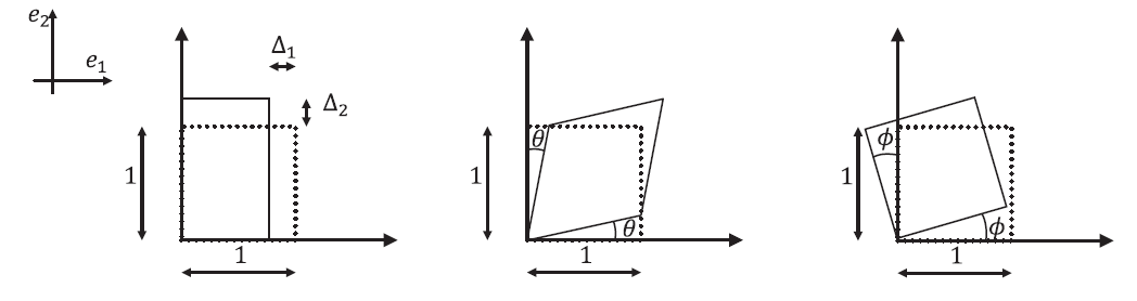
    • Write expressions for the displacement components and as functions of , , and the variables shown for each square.
    • Determine the components of the infinitesimal strain tensor and the infinitesimal rotation tensor.
    • Determine the components of the Green strain tensor.