Engineering at Alberta Courses » Combined Hardening

Mathematical Modelling of Plasticity: Combined Hardening

Strain Decomposition and Incremental Behaviour in Multi-axial Stress State with Combined Kinematidc and Isotropic Hardening (Bauschinger Effect)

In order to include the Bauschinger effect, various modifications to the isotropic hardening models presented in the previous section have been proposed throughout the development of the theory. The most successful and generalized form is that of the combined nonlinear kinematic and isotropic hardening model. In this section, the general form for this material model is presented.

Uniaxial Stress State Representation

In a uniaxial state of stress, modelling the Bauschinger effect is implemented by assuming that the difference between the yield stress in tension and in compression is due to the shifting of the yield surface by a value that is equal to $\overline{\alpha}$ , which is termed the backstress. The yield stress $\sigma_Y$ is assumed to be the sum of two components: $\sigma_{Y\alpha}$ which is the yield stress with respect to the shifted centre of the yield surface and $\overline{\alpha}$ which describes the shifting of the yield surface. Both $\sigma_{Y\alpha}$ and $\overline{\alpha}$ are assumed to be functions of the history of the deformation represented by $\overline{\varepsilon^p}$ and the values of the stress increment. Figure 11 shows the schematics of three different models that can be utilized to model the Bauschinger effect. In the first model (Figure 11a), referred to as the linear kinematic model, the yield stress with respect to the shifted centre $\sigma_{Y\alpha}$ is assumed to be constant while the shifting of the centre of the yield surface is assumed to be linear. This model can be enhanced by assuming that the $\sigma_{Y\alpha}$ varies with the equivalent plastic strain in a nonlinear fashion (Figure 11b). It is also possible to assume that the backstress follows a nonlinear relationship leading to the general nonlinear combined kinematic and isotropic hardening model, as shown in Figure 11c. 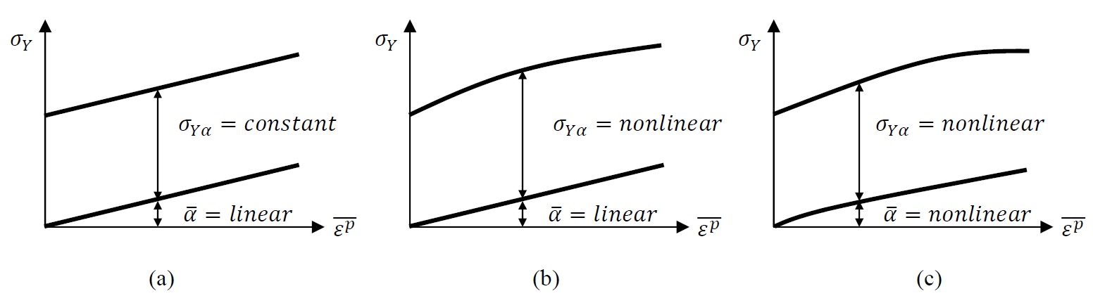Obviously, in order to calibrate such material model, numerous experiments have to be conducted to fit material curves for $\sigma_{Y\alpha}$ and for $\overline{\alpha}$ .

Figure 11. Three different models for the decomposition of the yield stress $\sigma_Y$ into a yield stress $\sigma_{Y\alpha}$ with respect to the centre of the yield surface and a backstress $\overline{\alpha}$ . (a) Kinematic hardening models, (b) combined linear kinematic hardening and nonlinear isotropic hardening model, (c) nonlinear kinematic and isotropic hardening model.

The most successful constitutive law model that describes the evolution of the backstress is the Armstrong-Frederick evolution law which in a uniaxial state of stress has the following form:

$\dot{\overline{\alpha}} = C \dot{\overline{\varepsilon^p}} -\gamma \overline{\alpha} \dot{\overline{\varepsilon^p}}$

or in incremental form:

$\Delta \overline{\alpha} = C\Delta \overline{\varepsilon^p} - \gamma \overline{\alpha} \Delta \overline{\varepsilon^p}$

Where $C$ and $\gamma$ are material constants. An earlier version of the above evolution law contained only the first term and was termed “Ziegler’s law”. Ziegler’s law had a limitation that $\overline{\alpha}$ would be unbounded and keeps increasing with the increase of the plastic strain $\varepsilon_{11}^p$ . The clever introduction of the term $\gamma \overline{\alpha}\dot{\overline{\varepsilon^p}}$ forces the value of $\overline{\alpha}$ to be bounded since integration of the above formula leads to:

$\int_0^{\overline{\alpha}} \frac{1}{C-\gamma \overline{\alpha}} d\overline{\alpha} = \int_0^{\overline{\varepsilon^p}} d\overline{\varepsilon^p} \Rightarrow = \frac{C}{\gamma} (1-e^{-\gamma \overline{\varepsilon^p}})$

Thus, at higher levels of $\overline{\varepsilon^p}$ the value of $\overline{\alpha}$ is bounded by the ratio of the material constants $\frac{C}{\gamma}$ .

Multi-axial Stress State Implementation

In order to implement the above relationships in a multi-axial stress state, the backstress is assumed to be a tensor $\alpha\in\mathbb{M}^3$ with components $\alpha_{ij}$ . The yield function in this case is given as follows:

$f(\sigma - \alpha) = \sigma_{vM}\Big|_{\sigma - \alpha} - \sigma_{Y\alpha}$

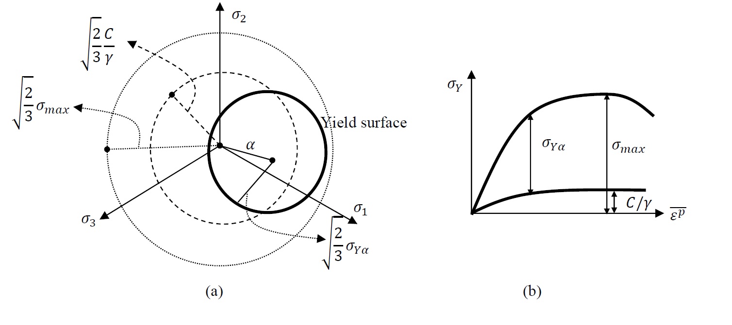
where $\sigma_{vM}|_{\sigma-\alpha}$ is the von Mises stress but with the difference $\sigma-\alpha$ substituted instead of the stress tensor $\sigma$ . Figure 12 shows the graphical representation of the yield function in the stress space of the principal stresses. If $\alpha^{dev}\in\mathbb{M}^3$ is the deviatoric backstress tensor, then, the yield function can be written as:

$f(\sigma - \alpha) = \sqrt{\sum_{i,j=1}^3 \frac{3}{2}(S_{ij} - \alpha_{ij}^{dev})(S_{ij} - \alpha_{ij}^{dev})}-\sigma_{Y\alpha}$

The Armstrong-Frederick material model describing the evolution of the backstress in a multi-axial stress state is given by the following form:

$\dot{\alpha_{ij}} = \Big(\frac{C(\sigma_{ij} - \alpha_{ij})}{\sigma_{Y\alpha}} - \gamma \alpha_{ij} \Big)^{\dot{\overline{\varepsilon^p}}}$

Or in incremental form:

$\Delta{\alpha_{ij}} = \Big(\frac{C(\sigma_{ij} - \alpha_{ij})}{\sigma_{Y\alpha}} - \gamma \alpha_{ij} \Big) \Delta \overline{\varepsilon^p}$

The bounding limit of $\alpha_{ij}$ is given by the value $\frac{C}{\gamma}$ and thus, the centre of the yield surface in the stress space is bounded by a cylinder of radius $\sqrt{\frac{2}{3}}\frac{C}{\gamma}$ , while the yield surface is bounded by the cylinder with a radius equal to $\sqrt{\frac{2}{3}}\sigma_{max}$ (Figure 12).

The associated flow rule can still be used for this material model where the plastic strain components are calculated as follows:

$\dot{\varepsilon_{ij}^p} = \dot{\overline{\varepsilon^p}} \frac{\partial \phi}{\partial \sigma_{ij}} = \dot{\overline{\varepsilon^p}} \Big(\frac{\frac{3}{2}(S_{ij}-\alpha_{ij}^{dev})}{\sigma_{vM}|_{\sigma-\alpha}}\Big)$

Or in incremental form:

$\Delta \varepsilon_{ij}^p = \Delta \overline{\varepsilon^p} \frac{\partial \phi}{\partial \sigma_{ij}} = \Delta\overline{\varepsilon^p} \Big(\frac{\frac{3}{2}(S_{ij}-\alpha_{ij}^{dev})}{\sigma_{vM}|_{\sigma-\alpha}}\Big)$

The increment in the plastic strain parameter can be obtained from the consistency condition as follows:

$\dot f = \sum_{i,j=1}^3 \frac{\partial f}{\partial \sigma_{ij}} \dot{\sigma_{ij}} + \sum_{i,j=1}^3 \frac{\partial f}{\partial \sigma_{ij}} \dot{\sigma_{ij}} - \frac{d\sigma_{Y\alpha}}{d\overline{\varepsilon^p}} \dot{\overline{\varepsilon^p}} = 0$

or in incremental form:

$\Delta f = \sum_{i,j=1}^3 \frac{\partial f}{\partial \sigma_{ij}} \Delta \sigma_{ij} + \sum_{i,j=1}^3 \frac{\partial f}{\partial \sigma_{ij}} \Delta \sigma_{ij} - \frac{d\sigma_{Y\alpha}}{d\overline{\varepsilon^p}} \Delta \overline{\varepsilon^p} = 0$

With

$\frac{\partial f}{\partial \sigma_{ij}} = -\frac{\partial f}{\partial \alpha_{ij}} = \frac{\frac{3}{2}(S_{ij} - \alpha_{ij}^{dev})}{\sigma_{vM}|_{\sigma - \alpha}}$