Engineering at Alberta Courses » Beams Under Axial Loading

Plane Beam Approximations: Beams Under Axial Loading

Learning Outcomes

Reproduce the derivation of the equilibrium equation of a beam under axial loading.
Describe the three basic assumptions for the equilibrium equation of beam under axial load.
Compute the normal force, the stress distribution, and the strain distribution in a beam by solving the differential equation of equilibrium.

The Euler Bernoulli and the Timoshenko beam formulations described account only for the deformations due to bending, without considering any axial deformation in the neutral axis of the beam. It is possible to augment the Euler Bernoulli and the Timoshenko beams so that they also account for axial deformations of the neutral axis, but because of the assumption of small deformations, the resulting equations of axial-loading deformations and bending deformations are uncoupled. i.e., the axial loading is only related to the axial deformation, and the lateral loading is only related to the lateral deformation. This uncoupling is only valid for small deformations. However, for large deformations, and normal force in an axially loaded beam can affect the lateral deformation as well. For example, phenomena such as buckling can only be modelled when the interaction between the axial loads and the lateral deformations are coupled.

Deformation Assumption

Under an axial load, a beam is assumed to deform such that the horizontal displacement is a smooth function $u_1=u_1(X_1)$ and that cross sections remain plane during the deformation (Figure 7). The effect of Poisson’s ratio is usually neglected. Thus, the position vector function is:

$x=\left(\begin{array}{c}X_1+u_1\\X_2\\X_3\end{array}\right)$

In this case, the displacement function is:

$u=x-X=\left(\begin{array}{c}u_1\\0\\0\end{array}\right)$

Since $u_1$ is a function of only $X_1$ , the only nonzero component of the strain is $\varepsilon_{11}$ :

$\varepsilon=\left(\begin{matrix}\frac{\mathrm{d}u_1}{\mathrm{d}X_1}&0&0\\0&0&0\\0&0&0\end{matrix}\right)$

On any cross section, $X_1$ is constant and therefore the values of $u_1$ and its derivatives are constant. Therefore, $\varepsilon_{11}$ is constant on any cross section perpendicular to $X_1$ .

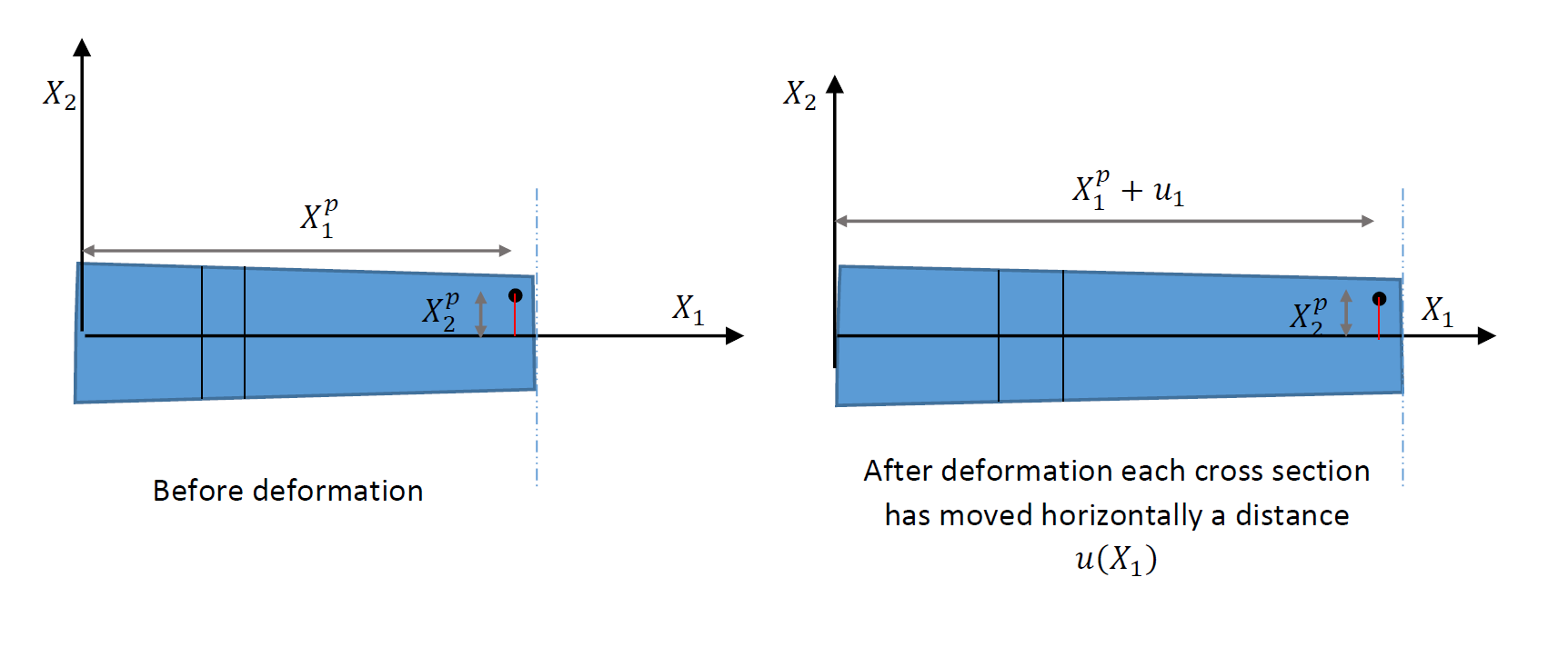BeamDeformationNormal — Figure 7. Deformation assumption of beams under axial loading. Cross section perpendicular to the neutral axis move horizontally in the direction of $X_1$ a distance $u_1(X_1)$ .

Equilibrium Equation

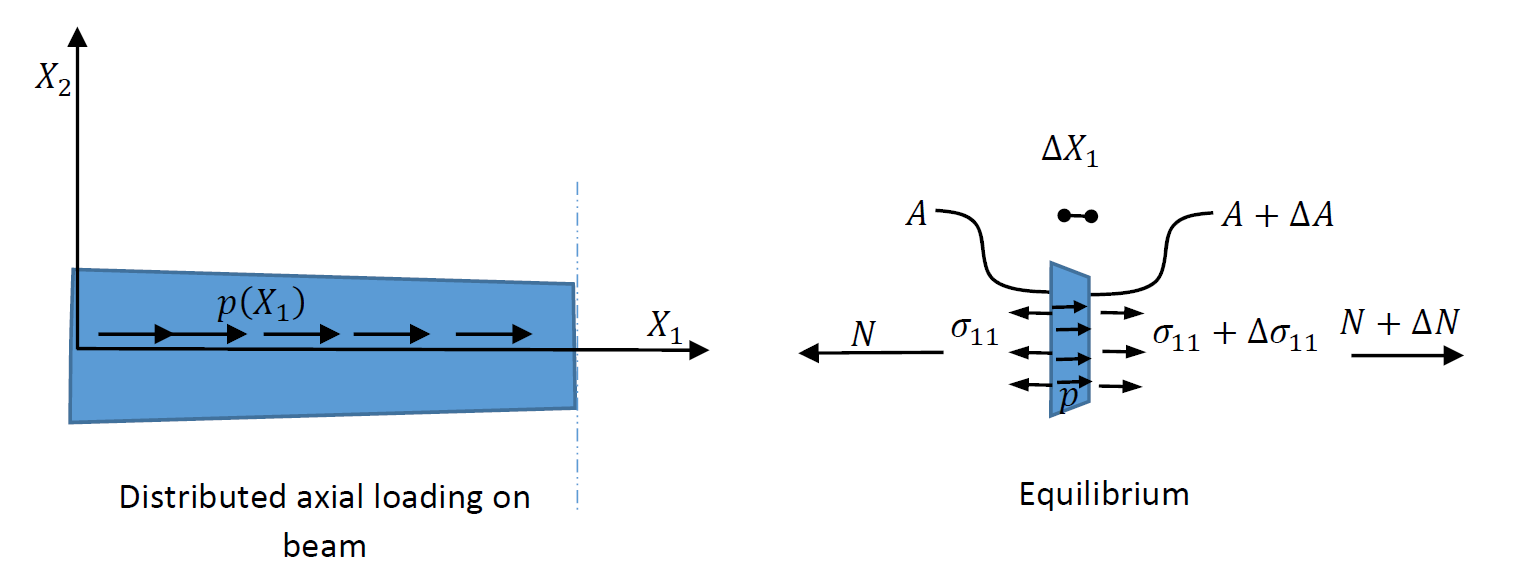
The beam is assumed to be under a distributed normal load of value p of units of force/unit length. Figure 8 shows the applied distributed load along with the equilibrium of a beam slide of length $\Delta X_1$ . The equilibrium equation can be written in terms of the normal force $N$ which is the integral of the stress component $\sigma_{11}$ over the cross sectional area:

$N=\int\int \! \sigma_{11}\,\mathrm{d}X_2\mathrm{d}X_3$

Since $\sigma_{11}$ is constant we have:

$N=\sigma_{11}A$

where $A$ is the cross sectional area. Equilibrium can be written by considering the three forces acting on the slice in Figure 8. The first force in $N+\Delta N$ acting on the right cross section and directed to the right. The second force is $N$ acting on the left cross section and directed to the left. The third is due to the distributed load $p$ . Therefore:

$\begin{split}F_1&=N+\Delta N = \sigma_{11}A+\frac{\partial N}{\partial X_1}\Delta X_1=\sigma_{11}A+\frac{\partial (\sigma_{11}A)}{\partial X_1}\Delta X_1\\F_2& =N=\sigma_{11}A\\F_3&=p\Delta X_1\end{split}$