
The Principle of Virtual Work: The Principle of Virtual Work
Learning Outcomes
- Identify that the principle of virtual work in a simple degree of freedom system is equivalent to static equilibrium.
- Apply the statement of the principle of virtual work in a continuum and in an Euler Bernoulli beam, and its extension to a beam under axial loading.
The principle of virtual work is widely used to solve a variety of continuum and solid mechanics problems. The statement of the principle of virtual work usually involves the phrase “virtual displacement field,” which is designed to engage the intuition by attempting to give a physical explanation to a mathematical statement. However, as will be shown in the following sections, the statement itself can be derived solely from mathematical, rather than physical explanations. In this section, the principle of virtual work will be presented for three applications. In the first, we will investigate the principle in its simplest form as it applies to a single degree of freedom. In the second and third, we will apply the principle to the continuum and to beams. The principle of virtual work itself is a different manifestation of the equilibrium equations, as it is an equivalent form of equilibrium. A system that is in equilibrium should satisfy the statement of the principle of virtual work and vice versa.
The Principle of Virtual Work For a Single Degree of Freedom
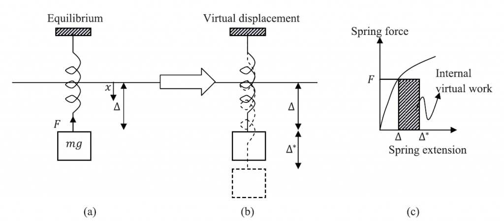
Consider the static equilibrium of a mass spring system. Assume that the force in the spring is a function of the displacement x of the spring, i.e.,  . At equilibrium, the sum of the vertical forces is equal to zero, and the force F in the spring is equal to the applied external load mg. Let the position of equilibrium be at
  (Figure 1). At equilibrium, we have:
![\[ F(x)|_{x=\Delta}=F(\Delta)=mg \]](https://engcourses-uofa.ca/wp-content/ql-cache/quicklatex.com-0bd7448e9b8a03422bce56d23d59f2b8_l3.png "Rendered by QuickLaTeX.com")
If the position of the spring is perturbed by an arbitrary small displacement  (Figure 1) and if the equilibrium equation above is multiplied by , then:
![\[ F(\Delta)\times\Delta^*=mg\times\Delta^* \]](https://engcourses-uofa.ca/wp-content/ql-cache/quicklatex.com-58a46392a52df08e2935979f062ead57_l3.png "Rendered by QuickLaTeX.com")
The above equation represents the statement of the principle of virtual work in a single degree of freedom system. From an equilibrium position, the external work done by the external forces mg during the application of a small virtual displacement is equal to the internal work done by the spring force during the application of that small virtual displacement (Figure 1).
The Principle of Virtual Work for a Continuum
In order to derive the equations of the virtual work, we start by the equilibrium equations in a continuum. Let  be the set representing a body in its reference configuration and
  be the set representing the body in its current configuration. Let
  be an orthonormal basis set, such that
  and
and  , each has coordinates:
  and
and  respectively. Let
  be the body forces vector map. The stresses at any point inside the body at static equilibrium satisfy the following equations:
(1) 
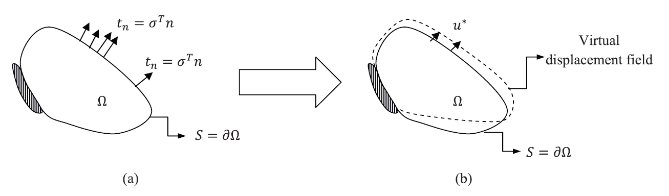
Let  be an arbitrary smooth function that could be viewed as a virtual displacement defined on
  (Figure 2). Let
  be the associated strain field defined as:
![\[ \varepsilon^*=\frac{1}{2}(\nabla u^*+\nabla (u^*)^T) \]](https://engcourses-uofa.ca/wp-content/ql-cache/quicklatex.com-de257b71a2b75c94c993e3ef034171df_l3.png "Rendered by QuickLaTeX.com")
and in component form:
![\[ \varepsilon_{ij}^*=\frac{1}{2}\left(\frac{\partial u_i^*}{\partial x_j}+\frac{\partial u_j^*}{\partial x_i}\right) \]](https://engcourses-uofa.ca/wp-content/ql-cache/quicklatex.com-36d93a1b210af7786c48e75d44484df0_l3.png "Rendered by QuickLaTeX.com")
When each of the equilibrium equations is multiplied by the corresponding component of the vector function  , and then the three equations are added together (in other words, if we take the dot product between the equilibrium equations as a vector and the vector ), the following equation is obtained
  :
:
(2) 
The following equality will be used:
![\[ \sum_{i,j=1}^3\frac{\partial \sigma_{ji}}{\partial x_j}u_i^*=\sum_{i,j=1}^3\left(\frac{\partial \sigma_{ji}u_i^*}{\partial x_j}-\sigma_{ji}\frac{\partial u_i^*}{\partial x_j}\right) \]](https://engcourses-uofa.ca/wp-content/ql-cache/quicklatex.com-d8f6a9e6cc413334dbb95aed87d02be5_l3.png "Rendered by QuickLaTeX.com")
Setting  and utilizing the symmetry of
  , Equation 2 can now be written as :
(3) 
In the next step, Equation 3 is integrated over the domain of . Therefore :
(4) 
Using the divergence theorem, the first volume integral can be replaced with a surface integral. Therefore, :
(5) 
Additionally, the Cauchy stress matrix is related to the external traction vectors on the surface of . Therefore, Equation 5 can be rewritten in the following form :
(6) 
(7) 
The left hand side is the external work done by the traction vectors  on the surface and the body forces vectors
  during a virtual smooth displacement field
  . The right hand side is equal to the internal work associated with the associated virtual strain field
  . The following are two important observations:
- The phrase (\forall u^*(x)) is necessary in the virtual work Equation (Equation 7).
- Equation 1 and Equation 7 are equivalent. You can derive Equation 1 by reversing the steps above from Equation 7.
The Principle of Virtual Work for an Euler Bernoulli Beam
The Euler Bernoulli beam is a special example of a continuum. We can either derive the equations from Equation 7 however, we will follow the same procedure above to obtain the virtual work equations for an Euler Bernoulli beam.
The equilibrium equation of an Euler Bernoulli beam is given by:
![\[ EI \frac{\mathrm{d}^4y}{\mathrm{d}X_1^4}=q \]](https://engcourses-uofa.ca/wp-content/ql-cache/quicklatex.com-171e3439ffb5961af03c2a7753366ffa_l3.png "Rendered by QuickLaTeX.com")
We can assume a virtual smooth displacement field  and proceed by multiplying the equilibrium equation by and integrate over the length of the beam. Therefore,
 :
:
![\[ \int_0^L \! EI \frac{\mathrm{d}^4y}{\mathrm{d}X_1^4} y^*\, \mathrm{d}X_1= \int_0^L \! qy^* \,\mathrm{d}X_1 \]](https://engcourses-uofa.ca/wp-content/ql-cache/quicklatex.com-f3589526151afff11ba110c8fe26b898_l3.png "Rendered by QuickLaTeX.com")
By applying integration by parts for the integral on the left hand side of the above equation, we get
![\[ EI\frac{\mathrm{d}^3y}{\mathrm{d}X_1^3}y^*\bigg|_0^L-\int_0^L \! EI \frac{\mathrm{d}^3y}{\mathrm{d}X_1^3} \frac{\mathrm{d}y^*}{\mathrm{d}X_1}\, \mathrm{d}X_1= \int_0^L \! qy^* \,\mathrm{d}X_1 \]](https://engcourses-uofa.ca/wp-content/ql-cache/quicklatex.com-80a77902fb8c0e3534397c11081d84b9_l3.png "Rendered by QuickLaTeX.com")
By applying integration by parts once more for the integral on the left hand side of the above equation, we get
![\[ EI\frac{\mathrm{d}^3y}{\mathrm{d}X_1^3}y^*\bigg|_0^L-EI\frac{\mathrm{d}^2y}{\mathrm{d}X_1^2}\frac{\mathrm{d}y^*}{\mathrm{d}X_1}\bigg|_0^L+\int_0^L \! EI \frac{\mathrm{d}^2y}{\mathrm{d}X_1^2} \frac{\mathrm{d}^2y^*}{\mathrm{d}X_1^2}\, \mathrm{d}X_1= \int_0^L \! qy^* \,\mathrm{d}X_1 \]](https://engcourses-uofa.ca/wp-content/ql-cache/quicklatex.com-76b9e7d39b41161583df98150e9590c5_l3.png "Rendered by QuickLaTeX.com")
Rearranging and utilizing the Euler Bernoulli beam equations for the shear and bending moments we reach the final virtual work expression:
(8) 
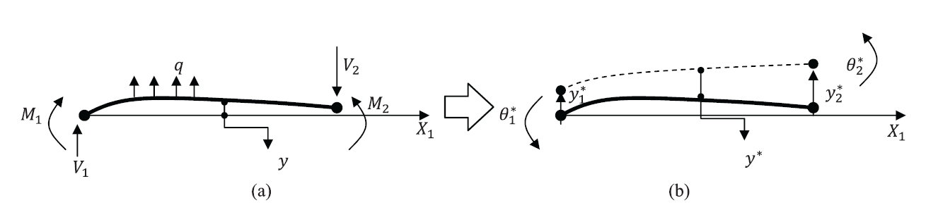
Where  , and
, and  are the boundary conditions for the shear, moment, virtual rotation and virtual displacement as shown in Figure 3. The right hand side represents the work done by the external forces during the application of a virtual smooth displacement field while the left hand side represents the internal work done by the bending moment during the application of the virtual displacement field.
The same notes regarding the principle of virtual work for a continuum apply to the Euler Bernoulli beam. The principle of virtual work equation is equivalent to the equilibrium equation. In addition, the phrase is an essential element of the principle of virtual work. I.e., the principle states that from an equilibrium position and under all possible virtual displacements, the internal virtual work is equal to the external virtual work.
are the boundary conditions for the shear, moment, virtual rotation and virtual displacement as shown in Figure 3. The right hand side represents the work done by the external forces during the application of a virtual smooth displacement field while the left hand side represents the internal work done by the bending moment during the application of the virtual displacement field.
The same notes regarding the principle of virtual work for a continuum apply to the Euler Bernoulli beam. The principle of virtual work equation is equivalent to the equilibrium equation. In addition, the phrase is an essential element of the principle of virtual work. I.e., the principle states that from an equilibrium position and under all possible virtual displacements, the internal virtual work is equal to the external virtual work.
The Principle of Virtual Work For a Timoshenko Beam
Similar to the Euler Bernoulli beam, we will assume a virtual arbitrary and smooth displacement field in addition to a virtual cross section shear deformation field  such that the total cross section virtual rotation is given by:
(9) 
Multiplying the equilibrium equation by and integrating over the length of the beam yields :
![\[ \int_0^L \! EI \frac{\mathrm{d}^3\psi}{\mathrm{d}X_1^3} y^*\, \mathrm{d}X_1= \int_0^L \! qy^* \,\mathrm{d}X_1 \]](https://engcourses-uofa.ca/wp-content/ql-cache/quicklatex.com-a7a86c91b4494962681dd9bd05813c14_l3.png "Rendered by QuickLaTeX.com")
Using integration by parts for the left hand side integral, :
![\[ EI\frac{\mathrm{d}^2\psi}{\mathrm{d}X_1^2}y^*\bigg|_0^L-\int_0^L \! EI \frac{\mathrm{d}^2\psi}{\mathrm{d}X_1^2} \frac{\mathrm{d}y^*}{\mathrm{d}X_1}\, \mathrm{d}X_1= \int_0^L \! qy^* \,\mathrm{d}X_1 \]](https://engcourses-uofa.ca/wp-content/ql-cache/quicklatex.com-ebc834dea444ae253ed9fa1701be5d37_l3.png "Rendered by QuickLaTeX.com")
Using Equation 9 to substitute for  yields
  :
:
![\[ EI\frac{\mathrm{d}^2\psi}{\mathrm{d}X_1^2}y^*\bigg|_0^L-\int_0^L \! EI \frac{\mathrm{d}^2\psi}{\mathrm{d}X_1^2} (\psi^*-\gamma^*)\, \mathrm{d}X_1= \int_0^L \! qy^* \,\mathrm{d}X_1 \]](https://engcourses-uofa.ca/wp-content/ql-cache/quicklatex.com-65e7fed342921a1bd796104226b98467_l3.png "Rendered by QuickLaTeX.com")
Applying the integration by parts to one of the integrals on the left hand side yields :
![\[ EI\frac{\mathrm{d}^2\psi}{\mathrm{d}X_1^2}y^*\bigg|_0^L-EI\frac{\mathrm{d}\psi}{\mathrm{d}X_1}\psi^*\bigg|_0^L+\int_0^L \! EI \frac{\mathrm{d}\psi}{\mathrm{d}X_1}\frac{\mathrm{d}\psi^*}{\mathrm{d}X_1} \, \mathrm{d}X_1+\int_0^L \! EI \frac{\mathrm{d}^2\psi}{\mathrm{d}X_1^2}\gamma^* \, \mathrm{d}X_1= \int_0^L \! qy^* \,\mathrm{d}X_1 \]](https://engcourses-uofa.ca/wp-content/ql-cache/quicklatex.com-b1e8034f07a9f0b5066229676b94412f_l3.png "Rendered by QuickLaTeX.com")
Finally, the statement of the virtual work principle has the following form :
![\[ \int_0^L \! EI \frac{\mathrm{d}\psi}{\mathrm{d}X_1}\frac{\mathrm{d}\psi^*}{\mathrm{d}X_1} \, \mathrm{d}X_1+\int_0^L \! V\gamma^* \, \mathrm{d}X_1= \int_0^L \! qy^* \,\mathrm{d}X_1-V_2y_2^*+V_1y_1^*+M_2\psi_2^*-M_1\psi_1^* \]](https://engcourses-uofa.ca/wp-content/ql-cache/quicklatex.com-45b85a102592cafec5b290eb592edc9e_l3.png "Rendered by QuickLaTeX.com")
Where  , and are the boundary conditions for the shear, moment, virtual cross section rotation and virtual displacement on ends 1 and 2. The right hand side represents the work done by the external forces during the application of a virtual smooth displacement field and a virtual smooth shear deformation field while the left hand side represents the internal work done by the bending moment and shear force during the application of the virtual displacement fields.
The same notes regarding the principle of virtual work for a continuum apply to the Timoshenko beam. The principle of virtual work equation is equivalent to the equilibrium equation. In addition, the phrase
, and are the boundary conditions for the shear, moment, virtual cross section rotation and virtual displacement on ends 1 and 2. The right hand side represents the work done by the external forces during the application of a virtual smooth displacement field and a virtual smooth shear deformation field while the left hand side represents the internal work done by the bending moment and shear force during the application of the virtual displacement fields.
The same notes regarding the principle of virtual work for a continuum apply to the Timoshenko beam. The principle of virtual work equation is equivalent to the equilibrium equation. In addition, the phrase  is an essential element of the principle of virtual work. I.e., the principle states that from an equilibrium position and under all possible virtual displacements, the internal virtual work is equal to the external virtual work.
Useful information with lucid explanation