FEA in One Dimension: One Dimensional Linear Elements

One Dimensional Linear Elements

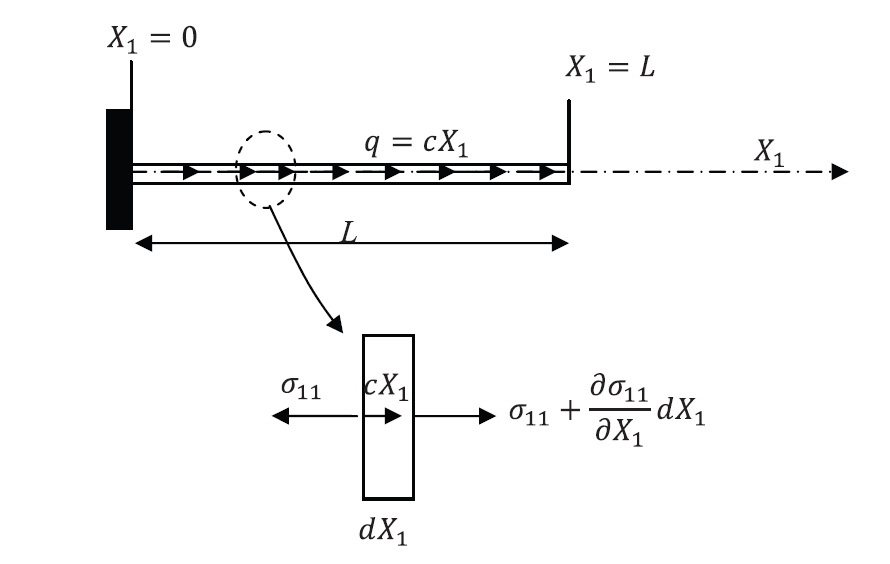
To illustrate the finite element method, we will start by solving the same example that was solved before using the Galerkin method but employing a finite element approximation. Using a four-piecewise linear trial function, find the approximate displacement function of the shown bar. Assume that the bar is linear elastic with Young’s modulus and cross-sectional area and that the small strain tensor is the appropriate measure of strain. Ignore the effect of Poisson’s ratio.

The different aspects of the finite element analysis method will be presented through solving this example as follows.

Shape Functions

In this example, a piecewise linear trial function for the displacement that satisfies the essential boundary condition is imposed. The displacement is interpolated between the four nodes and thus has the following form:

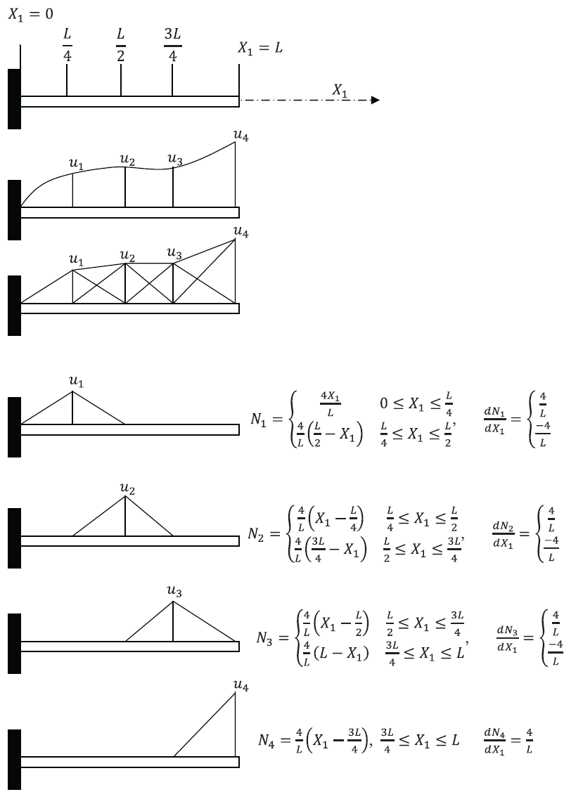
where are multipliers that happen to be the displacements at the nodes 1, 2, 3, and 4 respectively, while are the interpolation functions that have a value of 1 at node and decrease linearly to zero at the neighbouring nodes (Figure 3). These functions are traditionally termed the “hat” functions, for obvious reasons. They are also referred to as the shape functions since they define the shape of the deformation of the model. Except when they vanish, the shape functions have the form:

The derivatives of the shape functions are very simple and have the form:

Solution Using the Galerkin Method

The Galerkin method, involves equating the integral of the weighted residuals to zero. The weight functions are chosen as the functions which happen to be equal to the shape functions . After integration by parts as shown previously, the Galerkin method produces four equations of the form:

There are four trial or shape functions . Each appears only within a sub-interval and is equal to zero at the remaining part of the domain. Thus, the integration for each equation is only performed on the part where does not vanish.

Equation 1: vanishes every where except for . In this part of the domain, and vanish. Therefore, for the first equation we have:

Therefore, the first equation has the form:

The domain of integration can be updated to exclude the sub-domains when the integrand is equal to zero:

Equation 2: vanishes every where except for . In this part of the domain, vanishes. Therefore, for the second equation we have:

Therefore, the second equation has the form:

The domain of integration can be updated to exclude the sub-domains when the integrand is equal to zero:

Equation 3: vanishes every where except for . In this part of the domain, vanishes. Therefore, for the third equation we have:

Therefore, the third equation after excluding the sub-domains when the intgrand is equal to zero has the form:

Equation 4: vanishes every where except for . In this part of the domain, and vanish. Therefore, for the fourth equation we have:

Therefore, the fourth equation after excluding the sub-domains when the intgrand is equal to zero has the form:

The above four equations can be written in matrix form as follows:

where . The integration on both sides is relatively simple to calculate. The final equations have the following form:

which when solved gives the solution:

Comparison with the Exact Solution

The exact solution as shown previously is known and is equal to:

The exact displacement at the points 1, 2, 3, and 4 are given by:

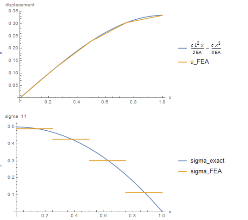
The finite element analysis approximation gave exact solution for the displacements of the points 1, 2, 3, and 4. However, in between those points, the finite element analysis approximation following linear interpolation. As shown in the figure below when setting , , , and units, the displacement values are almost accurate. However, the linear interpolation of the displacements means that the strain is constant in the area between points. Therefore, the stresses are constant between points and in fact, the stress distribution is discontinuous!

uexact = c*L^2/2/EA*x - c/6/EA*x^3;
N1 = Piecewise[{{4 x/L, 0 <= x <= L/4}, {4/L (L/2 - x), L/4 <= x <= L/2}}, 0];
N2 = Piecewise[{{4/L (x - L/4), L/4 <= x <= L/2}, {4/L (3 L/4 - x), L/2 <= x <= 3 L/4}}, 0];
N3 = Piecewise[{{4/L (x - L/2), L/2 <= x <= 3 L/4}, {4/L (L - x), 3 L/4 <= x <= L}}, 0];
N4 = Piecewise[{{4/L (x - 3 L/4), 3 L/4 <= x <= L}}, 0];
u1 = c*L^3/EA*(47/384);
u2 = c*L^3/EA*(11/48);
u3 = c*L^3/EA*(39/128);
u4 = c*L^3/EA*(1/3);
u = u1*N1 + u2*N2 + u3*N3 + u4*N4;
uexactp = uexact /. {c -> 1, EA -> 1, L -> 1}
sigmaexact = D[uexactp, x]
up = u /. {c -> 1, EA -> 1, L -> 1}
(*Assuming Young’s modulus = 1 unit *)
sigmap = D[up, x]
Plot[{uexactp, up}, {x, 0, 1}, AxesLabel -> {"x", "displacement"}, PlotLegends -> {uexact, u_FEA}]
Plot[{sigmaexact, sigmap}, {x, 0, 1}, AxesLabel -> {"x", "sigma_11"}, PlotLegends -> {"sigma_exact", "sigma_FEA"}]

import sympy as sp
import numpy as np
from sympy import lambdify
from matplotlib import pyplot as plt
x = sp.symbols("x")
xL = np.arange(0,1,0.01)
c,L,EA = 1,1,1
# Exact Calculations
u_exact = c*L**2/2/EA*x - c/sp.Rational("6")/EA*x**3
s_exact = u_exact.diff(x)
display("u_exact(x) =",u_exact,"s_exact(x) =",s_exact)
F = lambdify(x,u_exact)
dF = lambdify(x,s_exact)
y_exact = F(xL)
sy_exact = dF(xL)
def PN1(x):
    conds = [(x>=0)&(x<=L/4),(x>=L/4)&(x<L/2)]
    functions = [lambda x:4*x/L,lambda x:4/L*(L/2-x)]
    Dfunctions = [lambda x:4/L,lambda x:-4]
    return np.piecewise(x,conds,functions), np.piecewise(x,conds,Dfunctions)
def PN2(x):
    conds = [(x>=L/4)&(x<=L/2),(x>=L/2)&(x<3*L/4)]
    functions = [lambda x:4/L*(-L/4+x),lambda x:4/L*(3*L/4-x)]
    Dfunctions = [lambda x:4/L,lambda x:-4]
    return np.piecewise(x,conds,functions), np.piecewise(x,conds,Dfunctions)
def PN3(x):
    conds = [(x>=L/2)&(x<=3*L/4),(x>=3*L/4)&(x<=L)]
    functions = [lambda x:4/L*(-L/2+x),lambda x:4/L*(L-x)]
    Dfunctions = [lambda x:4/L,lambda x:-4]
    return np.piecewise(x,conds,functions), np.piecewise(x,conds,Dfunctions)
def PN4(x):
    conds = [(x>=3*L/4)&(x<=L)]
    functions = [lambda x:4/L*(-3*L/4+x)]
    Dfunctions = [lambda x:4/L]
    return np.piecewise(x,conds,functions), np.piecewise(x,conds,Dfunctions)
N1, DN1 = PN1(xL)
N2, DN2 = PN2(xL)
N3, DN3 = PN3(xL)
N4, DN4 = PN4(xL)
u1 = c*L**3/EA*(47/384)
u2 = c*L**3/EA*(11/48)
u3 = c*L**3/EA*(39/128)
u4 = c*L**3/EA*(1/3)
u = u1*N1+u2*N2+u3*N3+u4*N4
up = u1*DN1+u2*DN2+u3*DN3+u4*DN4
fig, ax = plt.subplots(2, figsize=(6,8))
ax[0].set_title("")
ax[0].set_xlabel("x")
ax[0].set_ylabel("displacement")
ax[0].plot(xL,y_exact,label="(c*L^2*x)/(2*EA) - (c*x^3)/(6*EA)")
ax[0].plot(xL,u,label="u_FEA")
ax[1].plot(xL,sy_exact,label="sigma_exact")
ax[1].plot(xL,up,label="sigma_FEA")
ax[1].set_ylabel("sigma11")
for i in ax:
    i.grid(True, which='both')
    i.axhline(y = 0, color = 'k')
    i.axvline(x = 0, color = 'k')
    i.set_xlabel("x")
    i.legend()

Solution Using the Virtual Work Method

As stated previously, the Galerkin method and the virtual work method are equivalent. The principle of virtual work states that, from a state of equilibrium, when a virtual admissible (compatible) displacement is applied, the increment in the work done by the external and body forces during the application of the virtual displacement is equal to the increment in the deformation energy stored. We will adopt the traditional matrix multiplication convention with differentiation between row and column vectors. The displacement function has the form:

The stress component due to the assumed trial displacement function has the following form:

The virtual displacement can be set by choosing virtual parameters :

Setting:

then the equations can be rewritten as follows:

The internal virtual work has the form:

The external virtual work has the form:

Equating the internal and external virtual work, the following is obtained:

where . Note that the factor is constant in this problem and was pulled out as a common factor for simplicity. Since the coefficients are arbitrary, the coefficients of each on both sides of the equality are equal. Therefore, the same equations of the Galerkin method are retrieved.

Elements, Nodes and Degrees of Freedom

In the finite element method, the domain is discretized into points which are called nodes and the regions between the nodes are called elements. The approximate solution involves assuming a trial function for the displacements interpolated between the values of the displacements the nodes. The displacement function is formed by multiplying the displacements of the nodes by shape functions. The displacements of the nodes are termed the degrees of freedom of the system. The right-hand side of the matrix equation formed is equivalent to a nodal force vector and is formed by lumping the distributed load and forming equivalent concentrated loads at the nodes.

For this particular example the solution is exact at the selected nodes. However, the solution within the elements will be linearly interpolated between the two values on each side and thus is not exact. The value of the gradient of the displacement at each node does not exist, as the displacement function is not differentiable at the nodes. In the finite element analysis method, the stresses that are related to the strains (the gradients of the displacements) are usually averaged at the nodes, and the degree of variation of the stresses between the different elements could be an indication of the accuracy of the solution. The matrix multiplied by the degrees of freedom is, in conservative systems, symmetric and is termed the stiffness matrix.

When the virtual work method was applied, the integration was done on the whole domain. However, it is possible to perform the integration locally on the elements. The equations of the virtual work can be written as follows:

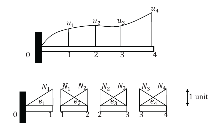
Because the integration can be done locally on the elements, it is possible to isolate the elements and perform the integration on each element separately (Figure 4). On each element, the shape functions or interpolation functions are associated with the end nodes. For example, element e2 connects nodes 1 and 2 with two shape functions, and . What is remarkable about the method is the similarity between all the elements shown in (Figure 4). Thus, a local stiffness matrix for each element can be developed, and then, the global stiffness matrix can be easily assembled by combining all the local stiffness matrices.

Element 1:

On element 1, the displacement is given by: and the virtual displacement is given by . By considering the first element, the first term (denoted ) in the internal virtual work equation has the following form:

is the local stiffness entry for element 1 corresponding to the degree of freedom . The first term in the external virtual work has the form:

where is the nodal force to be applied at node 1 corresponding to lumping the distributed load acting on element 1.

Element 2:

On element 2, the displacement is given by: and the virtual displacement is given by . By considering the second element, the second term in the internal virtual work equation has the following form:

where are the local stiffness matrix entries for element 2 corresponding to the degrees of freedom and . The second term in the external virtual work has the form:

where and are the nodal forces to be applied at nodes 1 and 2 corresponding to lumping the distributed load acting on element 2.

Element 3:

On element 3, the displacement is given by: and the virtual displacement is given by . By considering the third element, the third term in the internal virtual work equation has the following form:

where are the local stiffness matrix entries for element 3 corresponding to the degrees of freedom and . The third term in the external virtual work has the form:

where and are the nodal forces to be applied at nodes 2 and 3 corresponding to lumping the distributed load acting on element 3.

Element 4:

On element 4, the displacement is given by: and the virtual displacement is given by . By considering the fourth element, the fourth term in the internal virtual work equation has the following form:

where are the local stiffness matrix entries for element 4 corresponding to the degrees of freedom and . The fourth term in the external virtual work has the form:

where and are the nodal forces to be applied at nodes 3 and 4 corresponding to lumping the distributed load acting on element 4.

Global Stiffness Matrix
The global stiffness matrix can be assembled by the equation:

The resulting equations (global stiffness matrix and global nodal forces vector) considering the arbitrariness of the multipliers :

It is important to note that because the assumed displacement function satisfies the essential boundary conditions, the structure is stable, and the equations can be solved directly. In general, the structure under consideration would have five degrees of freedom and would have a global stiffness matrix and a global nodal forces vector. The nodal forces vector corresponding to the displacement of the first node where the displacement is prescribed would have an unknown reaction. The stiffness matrix can then be reduced into a matrix which can be solved.

Properties of the Stiffness Matrix

In the example above, the final equations had the following form:

where is the global stiffness matrix, is the vector of degrees of freedom while is the nodal forces vector. In general, the global stiffness matrix of an elastic structure formed using the finite element analysis method whether the problems has one, two, or three dimensions has the following properties:

• Sparsity: The stiffness matrix formed in the traditional finite element analysis is sparse, i.e., contains many zero entries. This property is due to the choice of piecewise-linear interpolation functions. The shape functions (or the interpolation functions) are chosen to be “Hat functions” that take values of 1 at each node and decrease linearly or in a parabolic fashion across the neighboring elements connected to that node. Nodes that are not connected together with any elements have a corresponding zero entry in the global stiffness matrix.

• Invertibility: (See the section on Invertible linear maps) The stiffness matrix of a structure is a linear map between and . Such map is invertible if and only if the map is injective (one to one), which means that the only element in the kernel of the map is the zero vector. Otherwise, if the map is not injective, then there are two nonzero distinct displacement vectors and that can be produced by the same force vector . I.e., , then the nonzero vector displacement can be applied to the structure without any external forces! If no boundary conditions are applied to a structure, then naturally rigid body motions and rigid body rotations can be applied without any external forces. Therefore, a stiffness matrix of a structure that is not restrained is not invertible and its determinant is equal to zero. Once enough boundary conditions are applied to the structure, then the only element of the kernel of the linear map is the zero element, the stiffness matrix is invertible, and its determinant is not equal to zero. Notice, however, that when a structure is not well supported and does not have the correct boundary conditions, the stiffness matrix is termed “ill conditioned”. Some finite element analysis software will still be able to find a possible solution, depending on the solution method. A user should be cautious in such cases since the solution could involve very large numbers for the displacement that would render the solution inaccurate.

• Symmetry: The stiffness matrix of an elastic structure is symmetric. The symmetry is a direct consequence of elasticity. Elasticity implies that there is an energy function such that . Therefore, implying that is symmetric.

• Positive and Semi-Positive Definiteness: (See the corresponding section in linear vector maps) A stable structure will deform in the direction of increasing external forces. Mathematically speaking, the dot product between the displacement and the force vectors has to be positive. If the structure is well restrained, i.e., is invertible, then is positive definite and any displacement field in the structure will produce positive energy. In mathematical terms, this imples: . However, if the structure is not well restrained, then is not invertible and such that . If the material of the structure is elastic, then the global stiffness matrix of the structure is semi-positive definite. Most finite element analysis software will check the invertibility of the stiffness matrix by finding the smallest eigenvalue of the stiffness matrix. If one of the eigenvalues of the stiffness matrix is zero, then the stiffness matrix is not invertible. If one of the eigenvalues is negative, then the stiffness matrix is not positive definite, since positive definiteness ensures positive eigenvalues (See the corresponding section in linear vector maps). A direct consequence of the positive definiteness is that the diagonal entries of the stiffness matrix have to be positive; since a diagonal element represents the force applied at the corresponding degree of freedom to produce unit displacement at this particular degree of freedom, then the requirement that the energy is positive ensures that the force and the displacement are in the same direction.

• Any vertical column of the stiffness matrix is equal to the vector of nodal forces required to move the corresponding degree of freedom by one unit displacement while keeping the remaining degrees of freedom equal to zero.

Video: