Engineering at Alberta Courses » Plasticity in Uniaxial Stress State

Mathematical Modelling of Plasticity: Plasticity in Uniaxial Stress State

In this section, the physical behaviour described previously will be modelled theoretically. Most of the equations in this section were initially developed by “curve fitting” to the behaviour and thus, mathematical idealizations are considered to simplify the relationships. The classical mathematical modelling of plasticity is formulated “incrementally” as shown in the following sections.

Yield Stress and Codes of Practice

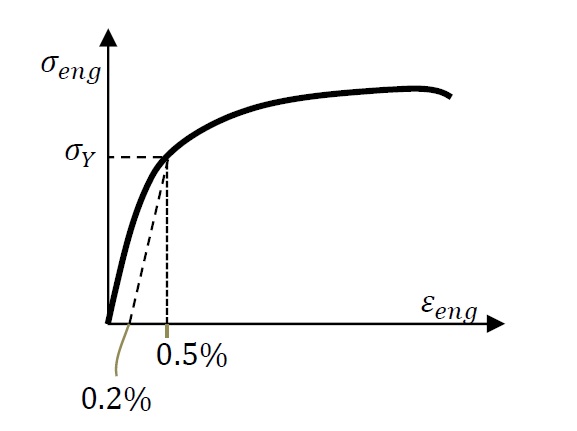
The yielding and strain hardening regions of the metal stress strain curve shown in Figure 1 are characterized by an increase in the “yield stress” with an increase in the amount of plastic deformation. While some metals, for example mild steel, exhibit a distinct “yield stress”, others have a more round stress strain curve with a gradual decrease in the slope of the curve between the stress and the strain. The yield stress in general is history dependent, i.e., it depends on the history of loading of the specimen and is not a unique function of the current state of stress. Codes of practice often prescribe three specified minimum values for the properties of a steel to be fit for a specific application. These are normally the “yield stress”, the “ultimate stress”, and the “elongation” corresponding to the failure point. The ultimate stress and the elongation associated with the filuare point can easily be obtained from any of the typical curves shown in Figure 2 , however, obtaining the exact elastic limit could be practically very difficult, and therefore, codes of practice often define the “yield stress” to be the stress corresponding to a specific value of strain (e.g. 0.005) or to the stress corresponding to the intersection between the 0.002 offset of the linear stress strain portion (Figure 4). The two criteria do not necessarily predict the same value for the yield stress $\sigma_Y$ .

Figure 4. Definition of yield stress or $\sigma_Y$ given by different codes of practice

Stress Strain Idealization

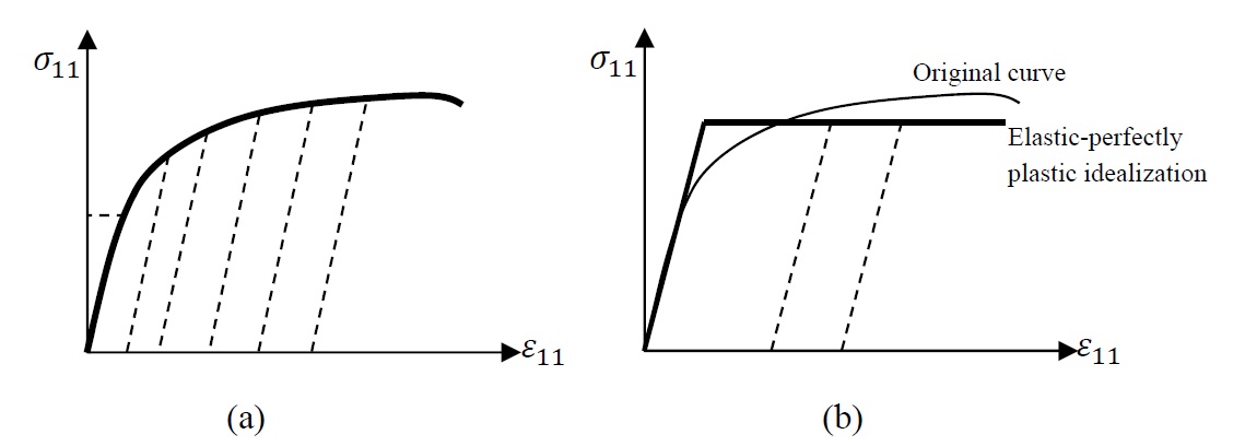
The relationship between the “true” stress versus the “true” or logarithmic strain is idealized to simplify the mathematical model. Points A and B are assumed to coincide and the loading and unloading in the yield and strain hardening region is assumed to follow a linear relationship as shown in Figure 5a. In other applications, especially those involving hand calculations or beam analysis, it is customary to assume an elastic-perfectly plastic stress strain curve, where the yield stress and the ultimate stress coincide (Figure 5b).

Figure 5. Different idealizations for the true stress versus true strain curves of metals: a) Unloading follows the dotted lines, b) elastic-perfectly plastic assumption with unloading following the dotted lines

Strain Decomposition and Incremental Behaviour in a Uniaxial Stress State

Upon removal of the applied load, metals exhibit what is referred to as permanent or plastic deformation. The true longitudinal strain can thus be decomposed into two components: an elastic component corresponding to the applied stress, and a permanent plastic deformation. In a uniaxial stress state where the force is applied along the direction of the basis vector $e_1$ , $\sigma_{11}$ corresponds to the true stress or the Cauchy stress component and $\varepsilon_{11}$ corresponds to the true longitudinal strain or logarithmic longitudinal strain along the direction of the basis vector $e_1$ . 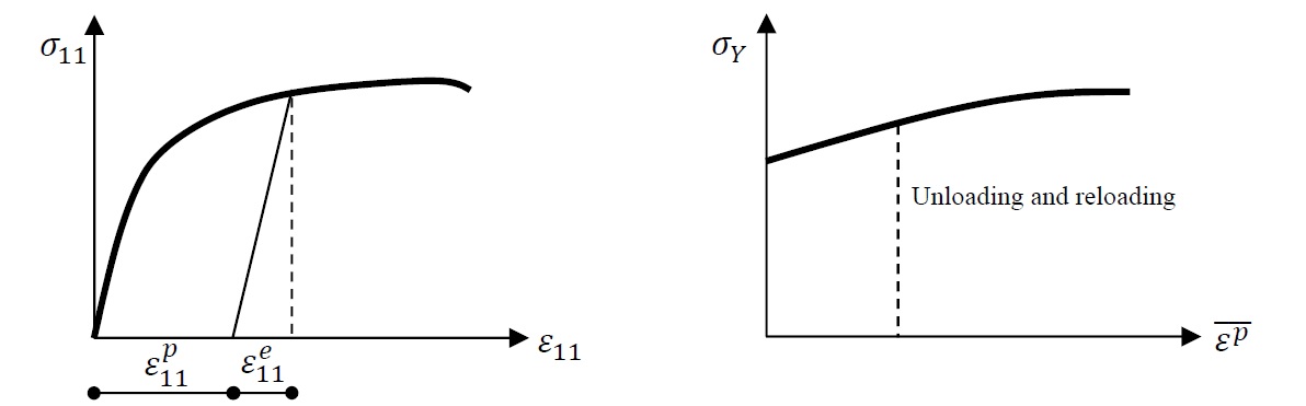The strain component can be decomposed into two components: an elastic component $\varepsilon_{11}^e$ and a plastic component $\varepsilon_{11}^p$ (Figure 6a). The elastic component is related to the stress using the linear elastic constitutive laws:

$\varepsilon_{11}^e = \frac{\sigma_{11}}{E}$

The plastic strain component can be obtained from the experimental results as follows:

$\varepsilon_{11}^p = \varepsilon_{11} - \frac{\sigma_{11}}{E}$

An explicit relationship describing the uniaxial stress component $\sigma_{11}$ and the plastic strain component $\varepsilon_{11}^p$ is often required (Figure 6b) for computations and thus a curve fitting model is often used. One of the very successful models is the Ramberg-Osgood model that fits a power law to the relationship between stress and plastic strain by introducing two material constants k and n as follows:

$\varepsilon_{11}^p = k\Big(\frac{\sigma_{11}}{E}\Big)^n$

If an increment in the load is such that $\sigma_{11}$ is decreased, then the elastic strain component is decreased while the plastic strain component stays the same. If an increment in the load is such that $\sigma_{11}$ reaches $\sigma_{Y}$ , then an increase beyond $\sigma_{Y}$ will cause an increase in the plastic strain $\varepsilon_{11}^p$ . i.e., unloading and reloading would follow vertical lines in Figure 6b. Thus, the above relationship in fact describes the magnitude of the yield stress at a certain value of a plastic strain parameter $\overline{\varepsilon^p}\in\mathbb{R}$ and is more precisely written in the form:

$\overline{\varepsilon^p} = k(\frac{\sigma_{Y}}{E})^n$

The plastic strain parameter $\overline{\varepsilon^p}$ is a measure of the history of plastic deformation such that $\overline{\varepsilon^p}>0$ and is always increasing. The plastic strain parameter is also referred to as the equivalent plastic strain. The overbar is used to differentiate between the plastic strain parameter and the plastic strain tensor $\varepsilon^p\in\mathbb{M}^3$ .

Figure 6. a) Decomposition of the strain component $\varepsilon_{11}$ into an elastic and a plastic component. b) the relationship between the plastic strain component and the applied stress

The remaining elastic strain components $\varepsilon_{22}^e$ , $\varepsilon_{33}^e$ , $\cdots$ can be obtained from the relationship between the stress and the strain. The remaining plastic strain components can be obtained from the isochoric deformation assumption and thus:

$\varepsilon_{22}^p = \varepsilon_{33}^p = -0.5\varepsilon_{11}^p$

In the above idealization, three functions were implicitly presented to fully describe the constitutive law of the plasticity of metals. These are the yield function, the hardening rule and the flow rule. As plastic deformation is dependent on the history of the loading, these functions can be conveniently written in terms of one parameter that represents the loading history. This one parameter is chosen to be the value of $\overline{\varepsilon^p}$ The following section describes these three rules.

Yield Function

The yield function is the function that describes whether the material is about to exhibit plastic deformation or not. In a uniaxial state of stress, if $\sigma_{11}$ is less than $\sigma_{Y}$ then, the behaviour is elastic. Once $\sigma_{11}$ reaches $\sigma_{Y}$ then the material is about to exhibit plastic deformation. $\sigma_{11}$ can never be higher than $\sigma_{Y}$ since as $\sigma_{11}$ increases, $\sigma_{Y}$ increases as well. If the stress matrix of the uniaxial stress state is denoted by $\sigma$ , then the yield function can be defined as:

$f(\sigma) = \sigma_{11} - \sigma_{Y} (\overline{\varepsilon^p})$

If $f(\sigma)<0$ , then the material is exhibiting elastic deformations, while if $f(\sigma)=0$ then, the material is about to exhibit plastic strain. As the material exhibits plastic strain, the change in the applied stress has to be such that the new stress state mathematically lies on the yield surface, i.e.,

$\dot f (\sigma) = \dot \sigma_{11} - \frac{d\sigma_Y}{d \overline{\varepsilon^p}} \dot{\overline{\varepsilon^p}} = 0$

In other words, the rate of change of the stress components $\sigma_{11}$ is related to the rate of change of the equivalent plastic strain $\overline{\varepsilon^p}$ . The above relationship is called the consistency condition. Traditionally, the consistency condition is written in the following incremental form:

$\Delta f = \Delta \sigma_{11} - \Delta \sigma_Y = \Delta \sigma_{11} - \frac{d\sigma_Y}{d\overline{\varepsilon^p}} \Delta \overline{\varepsilon^p} = 0$

The incremental form relates the increment in the increase in the applied stress to the incremental change of the yield stress of the material, or the increment in the applied stress to the increment in the plastic strain parameter. The incremental form represents a numerical integration scheme by which the increments in $\overline{\varepsilon^p}$ can be calculated as the applied stress is changed. The backward Euler numerical integration scheme is usually employed as it results in an approximation that is more accurate than the traditional forward Euler numerical integration scheme.

Hardening Rule

The hardening rule is the function that gives the value of the yield stress as a function of the history of the loading. A typical relationship obtained from experiments is shown in Figure 6b and can conveniently be represented by the Ramberg-Osgood approximation:

$\overline{\varepsilon^p} = k\Big(\frac{\sigma_Y}{E}\Big)^n$

This relationship is termed the hardening rule. Given the current amount of the accumulated plastic strain parameter $\overline{\varepsilon^p}$ in the material, the value of the yield stress $\sigma_Y$ is obtained.

Flow Rule

The flow rule is the function that dictates the amount of plastic strain that will accumulate during an increment in the loading. For a uniaxial state of stress the rate of change of the plastic strain aligned with the direction of the applied stress is equal to the rate of change of the plastic strain parameter (the equivalent plastic strain) $\dot{\varepsilon}_{11}^p=\dot{\overline{\varepsilon^p}}$ . The rate of change of the applied stress is equal to the rate of change of the yield stress, i.e,. $\dot{\sigma}_{11}=\dot{\sigma}_Y$ . Thus, the rates of change of $\varepsilon_{11}^p$ and $\sigma_{11}$ are related as follows:

$\dot{\varepsilon}_{11}^p = \frac{\dot{\sigma_{11}}}{\frac{d\sigma_Y}{d\overline{\varepsilon^p}}}$

In addition, the isochoric nature of the plastic deformation leads to the following relationship between the rates of change of the plastic strain components:

$\dot{\varepsilon}_{22}^p = \dot{\varepsilon}_{33}^p = -0.5\dot{\varepsilon}_{11}^p$

The above relationships can be written in incremental form such that $\Delta\varepsilon_{11}^p=\Delta\overline{\varepsilon^p}$ and $\Delta\sigma_{11}=\Delta\sigma_Y$ , then the increments in the plastic strain components are given by:

$\Delta \varepsilon_{11}^p = \frac{\Delta \sigma_{11}}{\frac{d\sigma_Y}{d \overline{\varepsilon^p}}}$

$\Delta \varepsilon_{22}^p = \Delta \varepsilon_{33}^p = -0.5\Delta \varepsilon_{11}^p$

The total value of the plastic strain components at the end of each increment is equal to the sum of all the plastic strain components increments developed throughout the loading. The backward Euler numerical integration scheme is usually employed for better accuracy.

Open Educational Resources