Engineering at Alberta Courses

Numerical Differentiation: Comparison

Comparison

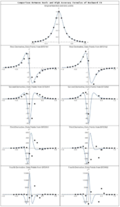
For the sake of comparison, data points generated by the Runge function $y=\frac{1}{1+25x^2}$ in the range $x\in[-1,1]$ are used to compare the different formulas obtained above. The exact first, second, third, and fourth derivatives of the function are plotted against the first, second, third, and fourth derivatives obtained using the formulas above. To differentiate between the results, the terms FFD, BFD, and CFD are used for forward, backward, and centred finite difference respectively. FFD1h1,FFD2h1, FFD3h1, and FFD4h1 indicate the forward finite difference first, second, third, and fourth derivatives respectively obtained using the basic formulas whose error terms are $\mathcal{O} (h)$ . The same applies for the basic formulas of the backward finite difference. However, CFD1h2, CFD2h2, CFD3h2, and CFD4h2 indicate the centred finite difference first, second, third, and fourth derivatives respectively obtained using the basic formulas whose error terms are $\mathcal{O}(h^2)$ . For higher accuracy formulas of the forward and backward finite difference, h1 is replaced by h2, while for higher accuracy formulas of the centred finite difference, h2 is replaced by h4. To generate these plots, the following Mathematica code was utilized. Given a table of data of two dimensions $(x_i,y_i)$ , the procedures in the code below provides the tables of the derivatives listed above. Note that the code below generates the data using the Runge function with a specific $h$ , but does not apply the procedure to the data. Click on the picture associated with each section to active the corresponding tool.

View Mathematica Code

h=0.1;
n = 2/h + 1;
y = 1/(1 + 25 x^2);
yp = D[y, x];
ypp = D[yp, x];
yppp = D[ypp, x];
ypppp = D[yppp, x];
Data = Table[{-1 + h*(i - 1), (y /. x -> -1 + h*(i - 1))}, {i, 1, n}];
FFD1h1[Data_] := (n = Length[Data]; h = Data[[2, 1]] - Data[[1, 1]]; f = Data[[All, 2]]; Table[{Data[[i, 1]], (f[[i + 1]] - f[[i]])/h}, {i, 1, n - 1}]);
FFD1h2[Data_] := (n = Length[Data]; h = Data[[2, 1]] - Data[[1, 1]]; f = Data[[All, 2]]; Table[{Data[[i, 1]], (-f[[i + 2]] + 4 f[[i + 1]] - 3 f[[i]])/2/h}, {i, 1, n - 2}]);
FFD2h1[Data_] := (n = Length[Data]; h = Data[[2, 1]] - Data[[1, 1]]; f = Data[[All, 2]];  Table[{Data[[i, 1]], (f[[i + 2]] - 2 f[[i + 1]] + f[[i]])/h^2}, {i, 1, n - 2}]);
FFD2h2[Data_] := (n = Length[Data]; h = Data[[2, 1]] - Data[[1, 1]]; f = Data[[All, 2]]; Table[{Data[[i,1]], (-f[[i + 3]] + 4 f[[i + 2]] - 5 f[[i + 1]] + 2 f[[i]])/ h^2}, {i, 1, n - 3}]);
FFD3h1[Data_] := (n = Length[Data]; h = Data[[2, 1]] - Data[[1, 1]];  f = Data[[All, 2]]; Table[{Data[[i,  1]], (f[[i + 3]] - 3 f[[i + 2]] + 3 f[[i + 1]] - f[[i]])/ h^3}, {i, 1, n - 3}]);
FFD3h2[Data_] := (n = Length[Data]; h = Data[[2, 1]] - Data[[1, 1]]; f = Data[[All, 2]]; Table[{Data[[i,  1]], (-3 f[[i + 4]] + 14 f[[i + 3]] - 24 f[[i + 2]] + 18 f[[i + 1]] - 5 f[[i]])/2/h^3}, {i, 1, n - 4}]);
FFD4h1[Data_] := (n = Length[Data]; h = Data[[2, 1]] - Data[[1, 1]]; f = Data[[All, 2]]; Table[{Data[[i, 1]], (f[[i + 4]] - 4 f[[i + 3]] + 6 f[[i + 2]] - 4 f[[i + 1]] +  f[[i]])/h^4}, {i, 1, n - 4}]);
FFD4h2[Data_] := (n = Length[Data]; h = Data[[2, 1]] - Data[[1, 1]];  f = Data[[All, 2]]; Table[{Data[[i,1]], (-2 f[[i + 5]] + 11 f[[i + 4]] - 24 f[[i + 3]] +  26 f[[i + 2]] - 14 f[[i + 1]] + 3 f[[i]])/h^4}, {i, 1,  n - 5}]);
BFD1h1[Data_] := (n = Length[Data]; h = Data[[2, 1]] - Data[[1, 1]]; f = Data[[All, 2]];  Table[{Data[[i, 1]], (f[[i]] - f[[i - 1]])/h}, {i, 2, n}]);
BFD1h2[Data_] := (n = Length[Data]; h = Data[[2, 1]] - Data[[1, 1]]; f = Data[[All, 2]];  Table[{Data[[i, 1]], (3 f[[i]] - 4 f[[i - 1]] + f[[i - 2]])/2/h}, {i, 3, n}]);
BFD2h1[Data_] := (n = Length[Data]; h = Data[[2, 1]] - Data[[1, 1]]; f = Data[[All, 2]];  Table[{Data[[i, 1]], (f[[i]] - 2 f[[i - 1]] + f[[i - 2]])/h^2}, {i, 3, n}]);
BFD2h2[Data_] := (n = Length[Data]; h = Data[[2, 1]] - Data[[1, 1]];  f = Data[[All, 2]];  Table[{Data[[i,  1]], (2 f[[i]] - 5 f[[i - 1]] + 4 f[[i - 2]] - f[[i - 3]])/ h^2}, {i, 4, n}]);
BFD3h1[Data_] := (n = Length[Data]; h = Data[[2, 1]] - Data[[1, 1]]; f = Data[[All, 2]];  Table[{Data[[i,  1]], (f[[i]] - 3 f[[i - 1]] + 3 f[[i - 2]] - f[[i - 3]])/ h^3}, {i, 4, n}]);
BFD3h2[Data_] := (n = Length[Data]; h = Data[[2, 1]] - Data[[1, 1]]; f = Data[[All, 2]];  Table[{Data[[i, 1]], (5 f[[i]] - 18 f[[i - 1]] + 24 f[[i - 2]] - 14 f[[i - 3]] + 3 f[[i - 4]])/2/h^3}, {i, 5, n}]);
BFD4h1[Data_] := (n = Length[Data]; h = Data[[2, 1]] - Data[[1, 1]]; f = Data[[All, 2]];  Table[{Data[[i,   1]], (f[[i]] - 4 f[[i - 1]] + 6 f[[i - 2]] - 4 f[[i - 3]] +  f[[i - 4]])/h^4}, {i, 5, n}]);
BFD4h2[Data_] := (n = Length[Data]; h = Data[[2, 1]] - Data[[1, 1]];  f = Data[[All, 2]];  Table[{Data[[i,  1]], (3 f[[i]] - 14 f[[i - 1]] + 26 f[[i - 2]] -   24 f[[i - 3]] + 11 f[[i - 4]] - 2 f[[i - 5]])/h^4}, {i, 6,  n}]);
CFD1h2[Data_] := (n = Length[Data]; h = Data[[2, 1]] - Data[[1, 1]];  f = Data[[All, 2]];  Table[{Data[[i, 1]], (f[[i + 1]] - f[[i - 1]])/2/h}, {i, 2,  n - 1}]);
CFD1h4[Data_] := (n = Length[Data]; h = Data[[2, 1]] - Data[[1, 1]];  f = Data[[All, 2]];  Table[{Data[[i,  1]], (-f[[i + 2]] + 8 f[[i + 1]] - 8 f[[i - 1]] + f[[i - 2]])/12/h}, {i, 3, n - 2}]);
CFD2h2[Data_] := (n = Length[Data]; h = Data[[2, 1]] - Data[[1, 1]]; f = Data[[All, 2]];  Table[{Data[[i, 1]], (f[[i + 1]] - 2 f[[i]] + f[[i - 1]])/h^2}, {i,2, n - 1}]);
CFD2h4[Data_] := (n = Length[Data]; h = Data[[2, 1]] - Data[[1, 1]]; f = Data[[All, 2]];  Table[{Data[[i, 1]], (-f[[i + 2]] + 16 f[[i + 1]] - 30 f[[i]] + 16 f[[i - 1]] -  f[[i - 2]])/12/h^2}, {i, 3, n - 2}]);
CFD3h2[Data_] := (n = Length[Data]; h = Data[[2, 1]] - Data[[1, 1]]; f = Data[[All, 2]];  Table[{Data[[i,  1]], (f[[i + 2]] - 2 f[[i + 1]] + 2 f[[i - 1]] - f[[i - 2]])/2/ h^3}, {i, 3, n - 2}]);
CFD3h4[Data_] := (n = Length[Data]; h = Data[[2, 1]] - Data[[1, 1]]; f = Data[[All, 2]];  Table[{Data[[i,  1]], (-f[[i + 3]] + 8 f[[i + 2]] - 13 f[[i + 1]] + 13 f[[i - 1]] - 8 f[[i - 2]] + f[[i - 3]])/8/h^3}, {i, 4, n - 3}]);
CFD4h2[Data_] := (n = Length[Data]; h = Data[[2, 1]] - Data[[1, 1]]; f = Data[[All, 2]]; Table[{Data[[i,  1]], (f[[i + 2]] - 4 f[[i + 1]] + 6 f[[i]] - 4 f[[i - 1]] +   f[[i - 2]])/h^4}, {i, 3, n - 2}]);
CFD4h4[Data_] := (n = Length[Data]; h = Data[[2, 1]] - Data[[1, 1]]; f = Data[[All, 2]]; Table[{Data[[i,   1]], (-f[[i + 3]] + 12 f[[i + 2]] - 39 f[[i + 1]] +   56 f[[i]] - 39 f[[i - 1]] + 12 f[[i - 2]] - f[[i - 3]])/6/ h^4}, {i, 4, n - 3}]);

View Python Code

import numpy as np
import sympy as sp

x = sp.symbols('x')
h = 0.1
n = int(2/h + 1)
y = 1/(1 + 25*x**2)
yp = y.diff(x, n=1)
ypp = yp.diff(x, n=2)
yppp = ypp.diff(x, n=3)
ypppp = yppp.diff(x, n=4)
Data = [[-1 + h*i, y.subs(x, -1 + h*i)] for i in range(n)]
def FFD1h1(Data): n = len(Data); Data = np.array(Data); h = Data[1,0] - Data[0,0]; f = Data[:,1]; return [[Data[i,0], (f[i + 1] - f[i])/h] for i in range(n - 1)]
def FFD1h2(Data): n = len(Data); Data = np.array(Data); h = Data[1,0] - Data[0,0]; f = Data[:,1]; return [[Data[i,0], (-f[i + 2] + 4*f[i + 1] - 3*f[i])/2/h] for i in range(n - 2)]
def FFD2h1(Data): n = len(Data); Data = np.array(Data); h = Data[1,0] - Data[0,0]; f = Data[:,1]; return [[Data[i,0], (f[i + 2] - 2*f[i + 1] + f[i])/h**2] for i in range(n - 2)]
def FFD2h2(Data): n = len(Data); Data = np.array(Data); h = Data[1,0] - Data[0,0]; f = Data[:,1]; return [[Data[i,0], (-f[i + 3] + 4*f[i + 2] - 5*f[i + 1] + 2*f[i])/h**2] for i in range(n - 3)]
def FFD3h1(Data): n = len(Data); Data = np.array(Data); h = Data[1,0] - Data[0,0]; f = Data[:,1]; return [[Data[i,0], (f[i + 3] - 3*f[i + 2] + 3*f[i + 1] - f[i])/h**3] for i in range(n - 3)]
def FFD3h2(Data): n = len(Data); Data = np.array(Data); h = Data[1,0] - Data[0,0]; f = Data[:,1]; return [[Data[i,0], (-3*f[i + 4] + 14*f[i + 3] - 24*f[i + 2] + 18*f[i + 1] - 5*f[i])/2/h**3] for i in range(n - 4)]
def FFD4h1(Data): n = len(Data); Data = np.array(Data); h = Data[1,0] - Data[0,0]; f = Data[:,1]; return [[Data[i,0], (f[i + 4] - 4*f[i + 3] + 6*f[i + 2] - 4*f[i + 1] + f[i])/h**4] for i in range(n - 4)]
def FFD4h2(Data): n = len(Data); Data = np.array(Data); h = Data[1,0] - Data[0,0]; f = Data[:,1]; return [[Data[i,0], (-2*f[i + 5] + 11*f[i + 4] - 24*f[i + 3] + 26*f[i + 2] - 14*f[i + 1] + 3*f[i])/h**4] for i in range(n - 5)]
def BFD1h1(Data): n = len(Data); Data = np.array(Data); h = Data[1,0] - Data[0,0]; f = Data[:,1]; return [[Data[i,0], (f[i] - f[i - 1])/h] for i in range(1, n)]
def BFD1h2(Data): n = len(Data); Data = np.array(Data); h = Data[1,0] - Data[0,0]; f = Data[:,1]; return [[Data[i,0], (3*f[i] - 4*f[i - 1] + f[i - 2])/2/h] for i in range(2, n)]
def BFD2h1(Data): n = len(Data); Data = np.array(Data); h = Data[1,0] - Data[0,0]; f = Data[:,1]; return [[Data[i,0], (f[i] - 2*f[i - 1] + f[i - 2])/h**2] for i in range(2, n)]
def BFD2h2(Data): n = len(Data); Data = np.array(Data); h = Data[1,0] - Data[0,0]; f = Data[:,1]; return [[Data[i,0], (2*f[i] - 5*f[i - 1] + 4*f[i - 2] - f[i - 3])/h**2] for i in range(3, n)]
def BFD3h1(Data): n = len(Data); Data = np.array(Data); h = Data[1,0] - Data[0,0]; f = Data[:,1]; return [[Data[i,0], (f[i] - 3*f[i - 1] + 3*f[i - 2] - f[i - 3])/h**3] for i in range(3, n)]
def BFD3h2(Data): n = len(Data); Data = np.array(Data); h = Data[1,0] - Data[0,0]; f = Data[:,1]; return [[Data[i,0], (5*f[i] - 18*f[i - 1] + 24*f[i - 2] - 14*f[i - 3] + 3*f[i - 4])/2/h**3] for i in range(4, n)]
def BFD4h1(Data): n = len(Data); Data = np.array(Data); h = Data[1,0] - Data[0,0]; f = Data[:,1]; return [[Data[i,0], (f[i] - 4*f[i - 1] + 6*f[i - 2] - 4*f[i - 3] + f[i - 4])/h**4] for i in range(4, n)]
def BFD4h2(Data): n = len(Data); Data = np.array(Data); h = Data[1,0] - Data[0,0]; f = Data[:,1]; return [[Data[i,0], (3*f[i] - 14*f[i - 1] + 26*f[i - 2] - 24*f[i - 3] + 11*f[i - 4] - 2*f[i - 5])/h**4] for i in range(5, n)]
def CFD1h2(Data): n = len(Data); Data = np.array(Data); h = Data[1,0] - Data[0,0]; f = Data[:,1]; return [[Data[i,0], (f[i + 1] - f[i - 1])/2/h] for i in range(1, n - 1)]
def CFD1h4(Data): n = len(Data); Data = np.array(Data); h = Data[1,0] - Data[0,0]; f = Data[:,1]; return [[Data[i,0], (-f[i + 2] + 8*f[i + 1] - 8*f[i - 1] + f[i - 2])/12/h] for i in range(2, n - 2)]
def CFD2h2(Data): n = len(Data); Data = np.array(Data); h = Data[1,0] - Data[0,0]; f = Data[:,1]; return [[Data[i,0], (f[i + 1] - 2*f[i] + f[i - 1])/h**2] for i in range(1, n - 1)]
def CFD2h4(Data): n = len(Data); Data = np.array(Data); h = Data[1,0] - Data[0,0]; f = Data[:,1]; return [[Data[i,0], (-f[i + 2] + 16*f[i + 1] - 30*f[i] + 16*f[i - 1] - f[i - 2])/12/h**2] for i in range(2, n - 2)]
def CFD3h2(Data): n = len(Data); Data = np.array(Data); h = Data[1,0] - Data[0,0]; f = Data[:,1]; return [[Data[i,0], (f[i + 2] - 2*f[i + 1] + 2*f[i - 1] - f[i - 2])/2/h**3] for i in range(2, n - 2)]
def CFD3h4(Data): n = len(Data); Data = np.array(Data); h = Data[1,0] - Data[0,0]; f = Data[:,1]; return [[Data[i,0], (-f[i + 3] + 8*f[i + 2] - 13*f[i + 1] + 13*f[i - 1] - 8*f[i - 2] + f[i - 3])/8/h**3] for i in range(3, n - 3)]
def CFD4h2(Data): n = len(Data); Data = np.array(Data); h = Data[1,0] - Data[0,0]; f = Data[:,1]; return [[Data[i,0], (f[i + 2] - 4*f[i + 1] + 6*f[i] - 4*f[i - 1] + f[i - 2])/h**4] for i in range(2, n - 2)]
def CFD4h4(Data): n = len(Data); Data = np.array(Data); h = Data[1,0] - Data[0,0]; f = Data[:,1]; return [[Data[i,0], (-f[i + 3] + 12*f[i + 2] - 39*f[i + 1] + 56*f[i] - 39*f[i - 1] + 12*f[i - 2] - f[i - 3])/6/h**4] for i in range(3, n - 3)]

The following are MATLAB codes that produce the comparisons below between the basic formulas.

MATLAB file comparison: Download

MATLAB file forward finite difference: Download

MATLAB file backward finite difference: Download

MATLAB file centred finite difference: Download

Basic Formulas

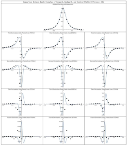
The following tool draws the plots of the exact first, second, third, and fourth derivatives of the Runge function overlaid with the data points of the first, second, third, and fourth derivatives obtained using the basic formulas for the forward, backward, and centred finite difference. You can click on the image to activate the tool. Choose $h=0.05$ and notice the following: in general, the centred finite difference scheme provides more accurate results, especially for the second and third derivatives. For all the formulas, accuracy is lost with the higher derivatives especially in the neighbourhood of $x=0$ where the function and its derivatives have large variations within a small region. The forward finite difference uses the function information on the right of the point to calculate the derivative and hence the calculated derivatives appear to be slightly shifted to the left in comparison with the exact derivatives. This is evident when looking at any of the derivatives. Similarly, the backward finite difference uses the function information on the left of the point to calculate the derivative and hence the calculated derivatives appear to be slightly shifted to the right in comparison with the exact derivatives. The centred finite difference scheme does not exhibit the same behaviour because it uses the information from both sides. When choosing $h\leq 0.01$ , the formulas provide very good approximation with the exact derivatives almost exactly overlaid with the finite difference calculations. However, for $h\geq 0.1$ , the results of the finite difference calculations for the higher derivatives are far from accurate in the neighbourhood of $x=0$ for the third and fourth derivatives.

Choose $h=0.1$ and notice that for the first derivative using forward finite difference, the derivative for the last point $x=1$ is unavailable (why?). Similarly, using the backward finite difference, the derivative for the first point $x=-1$ is unavailable. The derivatives for the first and last points are unavailable if the centred finite difference scheme is used. This carries on for the higher derivatives with the second, third, and fourth derivatives being unavailable for the last two, three, and four points when the forward finite difference scheme is used. The situation is reversed for the backward finite difference. The centred finite difference scheme provides more balanced results. The first and second derivatives at the first and last points are unavailable while the third and fourth derivatives at the first two points and the last two points are unavailable.

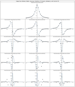
Higher Accuracy Formulas

The observations from the basic formulas carry over to the higher accuracy formulas except that the results are unavailable at a larger number of points on the edges of the domain. Choose $h=0.1$ and notice that the first derivative is unavailable at the last two points because the forward finite difference higher accuracy formulas use the information at $x_{i+2}$ to calculate the derivative at $x_i$ . Similarly, the first derivative is unavailable at the first two points in the backward finite difference higher accuracy formulas because the scheme uses the information at $x_{i-2}$ to calculate the derivative at $x_i$ . For higher derivatives, more results are unavailable at a larger number of points close to the edge of the domain. Similar to the basic formulas scheme, the centred finite difference provides more balanced results with the results being unavailable at the points on both edges of the domain.

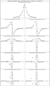
Forward Finite Difference

Both the basic formulas, and higher accuracy formulas for the forward finite difference scheme provide similar results. For $h>0.05$ , both schemes provide very good approximations for the first derivative, and for the flat parts of the higher derivatives. As explained above, the derivatives calculated using the formulas appear to be shifted to the left in comparison to the actual derivatives. For $h<0.01$ , both schemes provide relatively accurate predictions.

Backward Finite Difference

Both the basic formulas, and higher accuracy formulas for the backward finite difference scheme provide similar results. For $h>0.05$ , both schemes provides very good approximations for the first derivative, and for the flat parts of the higher derivatives. As explained above, the derivatives calculated using the formulas appear to be shifted to the right in comparison to the actual derivatives. For $h<0.01$ , both schemes provide relatively accurate predictions.

Centred Finite Difference

When $h<0.2$ , except for the fourth derivative at $x=0$ both centred finite difference schemes provide predictions that are very close to the exact results. It is obvious from these figures that when $h$ is relatively large, a centred finite difference scheme is perhaps more appropriate as it is more balanced and provides better accuracy. For smaller values of $h$ , all the schemes provide relatively acceptable predictions.