Engineering at Alberta Courses

Curve Fitting: Problems

The following data provides the number of trucks with a particular weight at each hour of the day on one of the busy US highways. The data is provided as , where is the hour and is the number of trucks: (1,16),(2,12),(3,14),(4,8),(5,24),(6,92),(7,311),(8,243),(9,558),(10,644),(11,768),(12,838),(13,911),(14,897),(15,853),(16,860),(17,853),(18,875),(19,673),(20,378),(21,207),(22,142),(23,108),(24,62). The distribution follows a Gaussian model of the form:
$N=a_1 e^{\frac{-(x-a_2)^2}{a_3}}$
- Find the parameters $a_1$ , $a_2$ , and $a_3$ that would produce the best fit to the data.
- On the same plot draw the model prediction vs. the data.
- Calculate the $R^2$ of the model.
- Calculate the sum of squares of the difference between the model prediction and the data.
In 2014, MacLeans published the following table showing the average tuition in Canadian provinces for the period from 2010 to 2014.
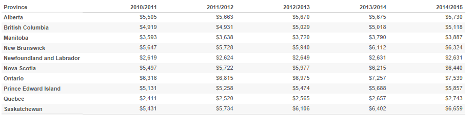
- Find the best linear model for each province that would predict tuition each year and its associated $R^2$ . Use calendar years to represent the $x$ axis data.
- Based on the linear fit, which province has the highest tuition increase per year and which one has the lowest?
The yield strength of steel decreases with elevated temperatures. The following experimental data provides the value of the temperature in 1000 degrees Celsius and the corresponding reduction factor in the yield strength. (0.05,1), (0.1,1), (0.2,0.95), (0.3,0.92), (0.4,0.82), (0.5,0.6), (0.6,0.4), (0.7,0.15), (0.8,0.15), (0.9,0.1), (1.0,0.1). Find the parameters $a_1, a_2, a_3, a_4, a_5$ in the following model that would provide the best fit to the data:
$R=a_1+\frac{a_2}{1+a_3 e^{\left(a_4x+a_5\right)}}$

Also, on the same plot draw the model prediction vs. the data. Based on the model, what is the reduction in the yield strength at temperatures of 150, 450, and 750 Degrees Celsius?
In order to noninvasively assess the stability of medical implants, Westover et al. devised a technique by which the implant is struck using a hand-piece while measuring the acceleration response.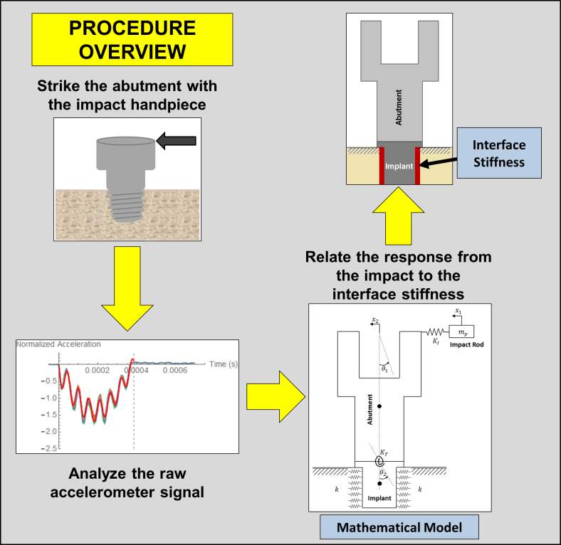In order to assess the stability, the acceleration $(a)$ data as a function of time $(t)$ has to be fit to a model of the form:
$\begin{split} y(t)&=a_1\sin{(a_2t+\phi_1)}+a_3e^{-a_4a_5t}\sin{\left(\sqrt{\left(1-a_4^2\right)}a_5t+\phi_2\right)}\\ a(t)&=\frac{\mathrm{d}^2y(t)}{\mathrm{d}t^2} \end{split}$

where $y(t)$ is the position, $a(t)$ is the acceleration, $a_1$ , $a_2$ , $a_3$ , $a_4$ , $a_5$ , $\phi_1$ , and $\phi_2$ are the model parameters. Initial guesses for the model parameters can be taken as: $1, 1500, 1, 0, 50000, 0.1, 0.1$ respectively.
The following text file OneStrike.txt contains the acceleration data collected by striking one of the implants. Download the data file and use the NonLinearModelFit built-in function to calculate the parameters for the best-fit model along with the value of $R^2$ . Plot the data overlapping the model.

Reference: L. Westover, W. Hodgetts, G. Faulkner, D. Raboud. 2015. Advanced System for Implant Stability Testing (ASIST). OSSEO 2015 5th International Congress on Bone Conduction Hearing and Related Technologies, Fairmont Chateau Lake Louise, Canada, May 20 – 23, 2015.
Find the parabola $y=a_0+a_1x+a_2x^2$ that best fits the following data:

x 2.2 1.1 -0.11 -1.1 -2.2

y 6.38 -1.21 -4.18 -3.63 1.65
Find the exponential model that best fits the following data:
data = {{10, 5.7}, {20, 18.2}, {30, 44.3}, {40, 74.5}, {50, 130.2}}
Find the power model that best fits the following data:
data = {{10, 5.7}, {20, 18.2}, {30, 44.3}, {40, 74.5}, {50, 130.2}}
Linear regression can be extended when the data depends on more than one variable (called multiple linear regression). For example, if the dependent variable is $z$ while the independent variables are $x$ and $y$ , then the data to be fitted have the form $(x_i,y_i,z_i)$ . In this case, the best-fit model is represented by a plane of the form $z=a_0+a_1x+a_2y$ . Using least squares assumption, find expressions for finding the coefficients of the model: $a_0$ , $a_1$ , and $a_2$ .

Open Educational Resources

Curve Fitting: Problems

Leave a Reply Cancel reply

x	2.2	1.1	-0.11	-1.1	-2.2
y	6.38	-1.21	-4.18	-3.63	1.65