
Ordinary Differential Equations: Solving Systems of IVPs
Solving Systems of IVPs
Many engineering problems contain systems of IVPs in which more than one dependent variable is a function of one independent variable, say  . For example, chemical reactions of more than one component are usually described using systems of IVPs in which the initial conditions are known. Similarly, the interaction of biological growth of different species (predators and prey) is usually represented by a system of IVPs in which the initial conditions are given. Generally, these systems can be represented as:
![\[\begin{split}\frac{\mathrm{d}x_1}{\mathrm{d}t}&=F_1(x_1,x_2,\cdots,x_n,t)\\\frac{\mathrm{d}x_2}{\mathrm{d}t}&=F_2(x_1,x_2,\cdots,x_n,t)\\&\vdots\\\frac{\mathrm{d}x_n}{\mathrm{d}t}&=F_n(x_1,x_2,\cdots,x_n,t)\end{split}\]](https://engcourses-uofa.ca/wp-content/ql-cache/quicklatex.com-22c12fe0a430fd90b72c47102c122559_l3.png "Rendered by QuickLaTeX.com")
The independent variable is discretized such that  with a constant step
  . In such systems, the initial conditions, namely the values of
  , are given. The values of
  when
when  are denoted:
  . In this case, the values of the dependent variables at
  can be obtained using the following system of equations:
![\[\begin{split}x_1^{(i+1)}&=x_1^{(i)}+\phi_1h\\x_2^{(i+1)}&=x_2^{(i)}+\phi_2h\\&\vdots\\x_n^{(i+1)}&=x_n^{(i)}+\phi_nh\\\end{split}\]](https://engcourses-uofa.ca/wp-content/ql-cache/quicklatex.com-e5dda044bd4f5ba870c24b058d1bed35_l3.png "Rendered by QuickLaTeX.com")
where
 depend on the method used. For example, if the explicit Euler method is used, then:
![\[\begin{split}\phi_1&=F_1(x_1^{(i)},x_2^{(i)},\cdots,x_n^{(i)},t_i)\\\phi_2&=F_2(x_1^{(i)},x_2^{(i)},\cdots,x_n^{(i)},t_i)\\&\vdots\\\phi_n&=F_n(x_1^{(i)},x_2^{(i)},\cdots,x_n^{(i)},t_i)\end{split}\]](https://engcourses-uofa.ca/wp-content/ql-cache/quicklatex.com-1a0d89d31fb044129ee5f4c758092f8b_l3.png "Rendered by QuickLaTeX.com")
Alternatively, if the classical Runge-Kutta method is used, then:
![\[\begin{split}\phi_1&=\frac{1}{6}(k_{11}+2k_{12}+2k_{13}+k_{14})\\\phi_2&=\frac{1}{6}(k_{21}+2k_{22}+2k_{23}+k_{24})\\&\vdots\\\phi_n&=\frac{1}{6}(k_{n1}+2k_{n2}+2k_{n3}+k_{n4})\end{split}\]](https://engcourses-uofa.ca/wp-content/ql-cache/quicklatex.com-3bd6807caf02eadc957fdd09d84f13b1_l3.png "Rendered by QuickLaTeX.com")
where
 ,
,  ,
,  , and
, and  are the
  values associated with the dependent variable
  and calculated according to the classical Runge-Kutta technique.
It should also be noted that higher-order IVPs can be solved by converting them into a system of first-order IVPs. For example, consider the IVP:
![\[\frac{\mathrm{d}^2x}{\mathrm{d}t^2}=F(x,t)\]](https://engcourses-uofa.ca/wp-content/ql-cache/quicklatex.com-97882419a777156187ca015009f03134_l3.png "Rendered by QuickLaTeX.com")
with the initial conditions
 and
and  given. Then, setting
  , the equation can be written as a system of two IVPs:
 ![\[\begin{split}\frac{\mathrm{d}x}{\mathrm{d}t}&=y\\\frac{\mathrm{d}y}{\mathrm{d}t}&=F(x,t)\end{split}\]](https://engcourses-uofa.ca/wp-content/ql-cache/quicklatex.com-ae0c5b101cbdf6ec9751ea0074922f91_l3.png "Rendered by QuickLaTeX.com")
with initial conditions given for
 and
and  .
.
Example
Consider the damped spring-mass mechanical system with  ,
,  with the initial conditions
  and
and  . Find the numerical solution for the position
  and the velocity
  for
for ![t\in[0,20]](https://engcourses-uofa.ca/wp-content/ql-cache/quicklatex.com-0002f8f3f7178b78ba8675785a19eb04_l3.png "Rendered by QuickLaTeX.com") using the explicit Euler method and the Runge-Kutta method. Use
using the explicit Euler method and the Runge-Kutta method. Use  .
.
Solution
The differential equation of the damped system is given by:
![\[\frac{\mathrm{d}^2x}{\mathrm{d}t^2}+0.15\frac{\mathrm{d}x}{\mathrm{d}t}+x=0\]](https://engcourses-uofa.ca/wp-content/ql-cache/quicklatex.com-8324f61b6f6f7638c2c443f2f278f863_l3.png "Rendered by QuickLaTeX.com")
The exact solution can be obtained analytically as:
![\[\begin{split}x&=-10e^{(-0.075t)}\left(\cos{(0.997184t)+0.0752118\sin{(0.997184t)}}\right)\\x'&=10.0282e^{(-0.075t)}\sin{(0.997184t)}\end{split}\]](https://engcourses-uofa.ca/wp-content/ql-cache/quicklatex.com-98a88a580a012cec9bf7fd53343dfb24_l3.png "Rendered by QuickLaTeX.com")
Notice that this is a second order ODE. To find the numerical solution, the equation will be converted into a system of 2 IVPs. Setting
, the equation can be converted into the following system: ![\[\begin{split}\frac{\mathrm{d}x}{\mathrm{d}t}&=y\\\frac{\mathrm{d}y}{\mathrm{d}t}&=-0.15y-x\\\end{split}\]](https://engcourses-uofa.ca/wp-content/ql-cache/quicklatex.com-99b66e1e4a84b1495b4cde315e1d4264_l3.png "Rendered by QuickLaTeX.com")
with the initial conditions and  . With , the interval can be split into
  time steps. The time discretization will be such that
  ,
,  ,
,  , up to
  . The corresponding positions are given by:
  while the corresponding velocities are given by:
  .
.
Explicit Euler Method
Using the explicit Euler method, the values of  and
and  can be evaluated as:
![\[\begin{split}x_{i+1}&=x_i+h\frac{\mathrm{d}x}{\mathrm{d}t}\bigg|_{(x_i,y_i,t_i)}=x_i+hy_i\\y_{i+1}&=y_i+h\frac{\mathrm{d}y}{\mathrm{d}t}\bigg|_{(x_i,y_i,t_i)}=y_i+h(-0.15y_i-x_i)\end{split}\]](https://engcourses-uofa.ca/wp-content/ql-cache/quicklatex.com-6aa9254d81827eebd352990513ba95e2_l3.png "Rendered by QuickLaTeX.com")
With the initial conditions
 and
and  , the values of
  and
and  at can be calculated as:
 ![\[\begin{split}x_1&=x_0+hy_0=-10+0.1(0)=-10\\y_1&=y_0+h(-0.15y_0-x_0)=0+0.1(-0.15\times0+10)=1\end{split}\]](https://engcourses-uofa.ca/wp-content/ql-cache/quicklatex.com-a0ed7f6c5c106bad1d38126128f9617d_l3.png "Rendered by QuickLaTeX.com")
Similarly, the values of
 and
and  can be obtained as:
 ![\[\begin{split}x_2&=x_1+hy_1=-10+0.1(1)=-9.9\\y_2&=y_1+h(-0.15y_1-x_1)=1+0.1(-0.15\times 1+10)=1.985\end{split}\]](https://engcourses-uofa.ca/wp-content/ql-cache/quicklatex.com-41febaae2230b10c6281c10e3ae54918_l3.png "Rendered by QuickLaTeX.com")
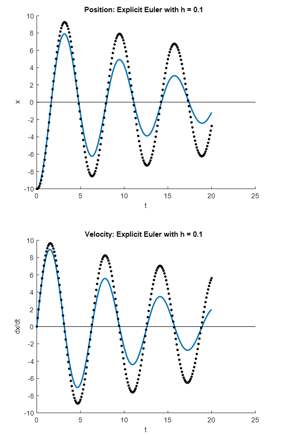
Proceeding iteratively, the values of and  up to
up to  can be obtained. The following figure shows the position (top) and velocity (bottom) obtained with the Explicit Euler method with (black dots) compared to the exact solution (blue line). The Microsoft Excel file EulerSystem.xlsx shows the obtained values.
Classical Runge-Kutta method
The two differential equations are designated  and
and  as follows:
![\[\begin{split}F_1(x,y,t)&=\frac{\mathrm{d}x}{\mathrm{d}t}=y\\F_2(x,y,t)&=\frac{\mathrm{d}y}{\mathrm{d}t}=-0.15y-x\end{split}\]](https://engcourses-uofa.ca/wp-content/ql-cache/quicklatex.com-9f404a09415a8d31a693fb1a64aca248_l3.png "Rendered by QuickLaTeX.com")
Using the classical Runge-Kutta method, the values of
and can be evaluated as: ![\[\begin{split}x_{i+1}&=x_i+\frac{h}{6}(k_{11}+2k_{12}+2k_{13}+k_{14})\\y_{i+1}&=y_i+\frac{h}{6}(k_{21}+2k_{22}+2k_{23}+k_{24}\end{split}\]](https://engcourses-uofa.ca/wp-content/ql-cache/quicklatex.com-7ff222019ec24a496a23f7b003f910ee_l3.png "Rendered by QuickLaTeX.com")
where:
![\[\begin{split}k_{11}&=F_1(x_i,y_i,t_i)=y_i\\k_{21}&=F_2(x_i,y_i,t_i)=-0.15y_i-x_i\\k_{12}&=F_1\left(x_i+\frac{h}{2}k_{11},y_i+\frac{h}{2}k_{21},t_i+\frac{h}{2}\right)=y_i+\frac{h}{2}k_{21}\\k_{22}&=F_2\left(x_i+\frac{h}{2}k_{11},y_i+\frac{h}{2}k_{21},t_i+\frac{h}{2}\right)=-0.15(y_i+\frac{h}{2}k_{21})-(x_i+\frac{h}{2}k_{11})\\k_{13}&=F_1\left(x_i+\frac{h}{2}k_{12},y_i+\frac{h}{2}k_{22},t_i+\frac{h}{2}\right)=y_i+\frac{h}{2}k_{22}\\k_{23}&=F_2\left(x_i+\frac{h}{2}k_{12},y_i+\frac{h}{2}k_{22},t_i+\frac{h}{2}\right)=-0.15(y_i+\frac{h}{2}k_{22})-(x_i+\frac{h}{2}k_{12})\\k_{14}&=F_1(x_i+hk_{13},y_i+hk_{23},t_i+h)=y_i+hk_{23}\\k_{24}&=F_2(x_i+hk_{13},y_i+hk_{23},t_i+h)=-0.15(y_i+hk_{23})-(x_i+hk_{13})\end{split}\]](https://engcourses-uofa.ca/wp-content/ql-cache/quicklatex.com-7b68cc7128ec4072a8b84b336ce5be6f_l3.png "Rendered by QuickLaTeX.com")
With the initial conditions
 and
and  , the values of
  can be calculated as:
 ![\[\begin{split}k_{11}&=y_0=0\\k_{21}&=-0.15y_0-x_0=10\\k_{12}&=y_0+\frac{h}{2}k_{21}=0+0.05\times 10=0.5\\k_{22}&=-0.15(y_0+\frac{h}{2}k_{21})-(x_0+\frac{h}{2}k_{11})\\&=-0.15(0+0.05\times 10)-(-10+0.05\times 0)=9.925\\k_{13}&=y_0+\frac{h}{2}k_{22}=0+0.05(9.925)=0.49625\\k_{23}&=-0.15(y_0+\frac{h}{2}k_{22})-(x_0+\frac{h}{2}k_{12})\\&=-0.15(0+0.05\times 9.925)-(-10+0.05\times 0.5)=9.90056\\k_{14}&=y_0+hk_{23}=0+0.1\times 9.90056=0.990056\\k_{24}&=-0.15(y_0+hk_{23})-(x_0+hk_{13})\\&=-0.15(0+0.1\times 9.90056)-(-10+0.1\times 0.49625)=9.80187\end{split}\]](https://engcourses-uofa.ca/wp-content/ql-cache/quicklatex.com-a3f7886e5b7cc5c0a2f7813ac930d824_l3.png "Rendered by QuickLaTeX.com")
Therefore:
![\[\begin{split}x_1&=x_0+\frac{h}{6}(k_{11}+2k_{12}+2k_{13}+k_{14})\\&=-10+\frac{0.1}{6}(0+2\times 0.5+2\times 0.49625+0.990056)=-9.9503\\y_1&=y_0+\frac{h}{6}(k_{21}+2k_{22}+2k_{23}+k_{24})\\&=0+\frac{0.1}{6}(10+2\times 9.925+2\times 9.90056+9.80187)=0.990883\end{split}\]](https://engcourses-uofa.ca/wp-content/ql-cache/quicklatex.com-2670507993deb7cccdd05ef55ae8f404_l3.png "Rendered by QuickLaTeX.com")
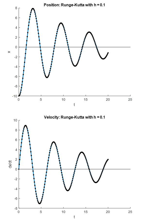
Proceeding iteratively, the values of
and up to can be obtained. The following figure shows the position (top) and velocity (bottom) obtained with the classical Runge-Kutta method with (black dots) compared to the exact solution (blue line). The Microsoft Excel file RK4System.xlsx shows the calculated up to the required time point.
Comparison
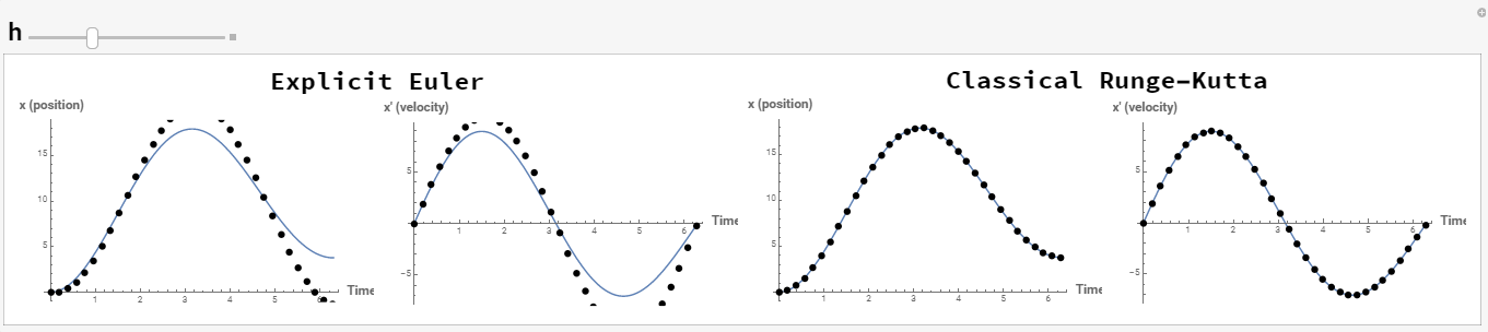
From the figures above, it is evident that using the explicit Euler method, the numerical solution deviates from the exact solution for higher values of . However, the classical Runge-Kutta method provides very accurate predictions.
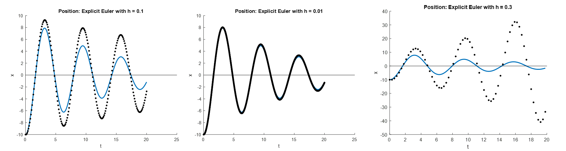
As shown in the figure below, the Explicit Euler method can produce results with higher accuracy using smaller values of the step size (i.e.  ). With higher values of the step size, the method can become unstable and grow without bound (i.e.
  ).
).
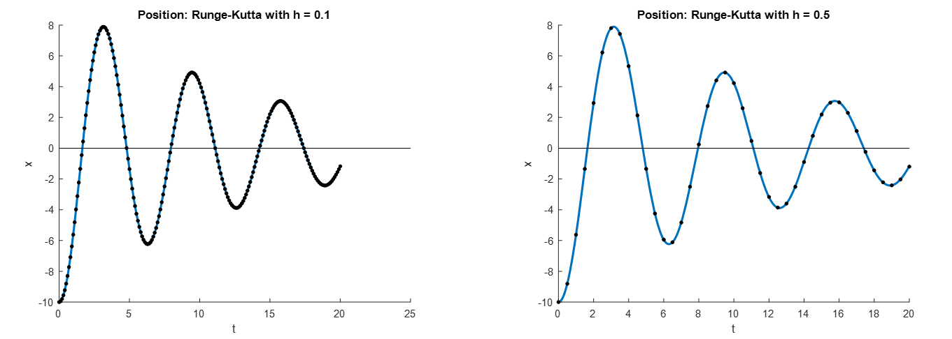
In contrast, the figure below demonstrates that the classical Runge-Kutta method is able to produce accurate results and maintain numerical stability for a step size as high as  .
.
The Mathematica code utilized to produce the curves is shown below.
View Mathematica CodeClear[x]
a = DSolve[{Derivative[2][x][t] == -(0.15*Derivative[1][x][t]) - x[t], Derivative[1][x][0] == 0, x[0] == -10}, x, t]
x = x[t] /. a[[1]]
xp = Simplify[D[x, {t}]]
Plot[x, {t, 0, 20}, AxesOrigin -> {0, 0}, AxesOrigin -> {0, 0}, AxesLabel -> {"time", "x (position)"}]
Plot[xp, {t, 0, 20}, AxesOrigin -> {0, 0}, AxesOrigin -> {0, 0}, AxesLabel -> {"time", "x' (velocity)"}]
EulerMethod2[fp1_, fp2_, x10_, x20_, h_, t0_, tmax_] := (n = (tmax - t0)/h + 1; x1table = Table[0, {i, 1, n}]; x2table = Table[0, {i, 1, n}]; x1table[[1]] = x10; x2table[[1]] = x20;
Do[x1table[[i]] = h*fp1[x1table[[i - 1]], x2table[[i - 1]], h*(i - 2) + t0] + x1table[[i - 1]]; x2table[[i]] = h*fp2[x1table[[i - 1]], x2table[[i - 1]], h*(i - 2) + t0] +
x2table[[i - 1]], {i, 2, n}]; Data = Table[{h*(i - 1) + t0, x1table[[i]], x2table[[i]]}, {i, 1, n}]; Data)
RK4Method2[fp1_, fp2_, x10_, x20_, h_, t0_, tmax_] := (n = (tmax - t0)/h + 1; x1table = Table[0, {i, 1, n}]; x1table[[1]] = x10; x2table = Table[0, {i, 1, n}]; x2table[[1]] = x20;
Do[k11 = fp1[x1table[[i - 1]], x2table[[i - 1]], h*(i - 2) + t0]; k21 = fp2[x1table[[i - 1]], x2table[[i - 1]], h*(i - 2) + t0];
k12 = fp1[(h*k11)/2 + x1table[[i - 1]], (h*k21)/2 + x2table[[i - 1]], h*(i - 1.5) + t0]; k22 = fp2[(h*k11)/2 + x1table[[i - 1]], (h*k21)/2 + x2table[[i - 1]], h*(i - 1.5) + t0];
k13 = fp1[(h*k12)/2 + x1table[[i - 1]], (h*k22)/2 + x2table[[i - 1]], h*(i - 1.5) + t0]; k23 = fp2[(h*k12)/2 + x1table[[i - 1]], (h*k22)/2 + x2table[[i - 1]], h*(i - 1.5) + t0];
k14 = fp1[h*k13 + x1table[[i - 1]], h*k23 + x2table[[i - 1]], h*(i - 1) + t0]; k24 = fp2[h*k13 + x1table[[i - 1]], h*k23 + x2table[[i - 1]], h*(i - 1) + t0];
x1table[[i]] = (1/6)*h*(k11 + 2*k12 + 2*k13 + k14) + x1table[[i - 1]]; x2table[[i]] = (1/6)*h*(k21 + 2*k22 + 2*k23 + k24) + x2table[[i - 1]], {i, 2, n}];
Data2 = Table[{h*(i - 1) + t0, x1table[[i]], x2table[[i]]}, {i, 1, n}]; Data2)
fp1[x_, y_, t_] := y;
fp2[x_, y_, t_] := -x - 0.15*y;
Data = EulerMethod2[fp1, fp2, -10, 0, 0.1, 0, 20];
DataPosition = Drop[Data, None, {3}];
DataVelocity = Drop[Data, None, {2}];
a1 = Plot[x, {t, 0, 20}, Epilog -> {PointSize[Large], Point[DataPosition]}, AxesOrigin -> {0, 0}, ImageSize -> Medium, AxesLabel -> {"Time", "x (position)"}];
a2 = Plot[xp, {t, 0, 20}, Epilog -> {PointSize[Large], Point[DataVelocity]}, AxesOrigin -> {0, 0}, ImageSize -> Medium, AxesLabel -> {"Time", "x' (velocity)"}];
a = Grid[{{a1, a2}}];
Grid[{{"Explicit Euler"}, {a}}]
Data = RK4Method2[fp1, fp2, -10, 0, 0.1, 0, 20];
DataPosition = Drop[Data, None, {3}];
DataVelocity = Drop[Data, None, {2}];
a1 = Plot[x, {t, 0, 20}, Epilog -> {PointSize[Large], Point[DataPosition]}, ImageSize -> Medium, AxesOrigin -> {0, 0}, AxesLabel -> {"Time", "x (position)"}];
a2 = Plot[xp, {t, 0, 20}, Epilog -> {PointSize[Large], Point[DataVelocity]}, ImageSize -> Medium, AxesOrigin -> {0, 0}, AxesLabel -> {"Time", "x' (velocity)"}];
a = Grid[{{a1, a2}}];
Grid[{{"Classical Runge-Kutta"}, {a}}]
View Python Code
# UPGRADE: need Sympy 1.2 or later, upgrade by running: "!pip install sympy --upgrade" in a code cell
# !pip install sympy --upgrade
import numpy as np
import sympy as sp
import matplotlib.pyplot as plt
sp.init_printing(use_latex=True)

x = sp.Function('x')
t = sp.symbols('t')
sol = sp.dsolve(x(t).diff(t,2) + x(t) + 0.15*x(t).diff(t), ics={x(0): -10, x(t).diff(t).subs(t,0): 0})
display(sol)
xp = sp.simplify(sol.rhs.diff(t))
display(xp)

x_val = np.arange(0,20,0.01)
plt.plot(x_val, [sol.subs(t, i).rhs for i in x_val])
plt.xlabel("time"); plt.ylabel("x (position)")
plt.grid(); plt.show()
plt.plot(x_val, [xp.subs(t, i) for i in x_val])
plt.xlabel("time"); plt.ylabel("x' (velocity)")
plt.grid(); plt.show()

def EulerMethod2(fp1, fp2, x10, x20, h, t0, tmax):
  n = int((tmax - t0)/h + 1)
  x1table = [0 for i in range(n)]
  x2table = [0 for i in range(n)]
  x1table[0] = x10
  x2table[0] = x20
  for i in range(1,n):
    x1table[i] = x1table[i - 1] +  h*fp1(x1table[i - 1], x2table[i - 1], t0 + (i - 1)*h)
    x2table[i] = x2table[i - 1] +  h*fp2(x1table[i - 1], x2table[i - 1], t0 + (i - 1)*h)
  Data = [[t0 + i*h, x1table[i], x2table[i]] for i in range(n)]
  return Data

def RK4Method2(fp1, fp2, x10, x20, h, t0, tmax):
  n = int((tmax - t0)/h + 1)
  x1table = [0 for i in range(n)]
  x1table[0] = x10
  x2table = [0 for i in range(n)]
  x2table[0] = x20
  for i in range(1,n):
    k11 = fp1(x1table[i - 1], x2table[i - 1], t0 + (i - 1)*h)
    k21 = fp2(x1table[i - 1], x2table[i - 1], t0 + (i - 1)*h)
    k12 = fp1(x1table[i - 1] + h/2*k11, x2table[i - 1] + h/2*k21, t0 + (i - 0.5)*h)
    k22 = fp2(x1table[i - 1] + h/2*k11, x2table[i - 1] + h/2*k21, t0 + (i - 0.5)*h)
    k13 = fp1(x1table[i - 1] + h/2*k12, x2table[i - 1] + h/2*k22, t0 + (i - 0.5)*h)
    k23 = fp2(x1table[i - 1] + h/2*k12, x2table[i - 1] + h/2*k22, t0 + (i - 0.5)*h)
    k14 = fp1(x1table[i - 1] + h*k13, x2table[i - 1] + h*k23, t0 + i*h)
    k24 = fp2(x1table[i - 1] + h*k13, x2table[i - 1] + h*k23, t0 + i*h)
    x1table[i] = x1table[i - 1] + h*(k11 + 2*k12 + 2*k13 + k14)/6
    x2table[i] = x2table[i - 1] + h*(k21 + 2*k22 + 2*k23 + k24)/6
  Data = [[t0 + i*h, x1table[i], x2table[i]] for i in range(n)]
  return Data

def fp1(x, y, t): return y
def fp2(x, y, t): return -x - 0.15*y
x_val = np.arange(0,20,0.01)

Data = EulerMethod2(fp1, fp2, -10, 0, 0.1, 0, 20)
plt.title("Explicit Euler")
plt.plot(x_val, [sol.subs(t, i).rhs for i in x_val])
plt.scatter([DataPosition[0] for DataPosition in Data],
            [DataPosition[1] for DataPosition in Data],c='k')
plt.xlabel("Time"); plt.ylabel("x (position)")
plt.grid(); plt.show()
plt.title("Explicit Euler")
plt.plot(x_val, [xp.subs(t, i) for i in x_val])
plt.scatter([DataVelocity[0] for DataVelocity in Data],
            [DataVelocity[2] for DataVelocity in Data],c='k')
plt.xlabel("Time"); plt.ylabel("x' (velocity)")
plt.grid(); plt.show()

Data = RK4Method2(fp1, fp2, -10, 0, 0.1, 0, 20)
plt.title("Classical Runge-Kutta")
plt.plot(x_val, [sol.subs(t, i).rhs for i in x_val])
plt.scatter([DataPosition[0] for DataPosition in Data],
            [DataPosition[1] for DataPosition in Data],c='k')
plt.xlabel("Time"); plt.ylabel("x (position)")
plt.grid(); plt.show()
plt.title("Classical Runge-Kutta")
plt.plot(x_val, [xp.subs(t, i) for i in x_val])
plt.scatter([DataVelocity[0] for DataVelocity in Data],
            [DataVelocity[2] for DataVelocity in Data],c='k')
plt.xlabel("Time"); plt.ylabel("x' (velocity)")
plt.grid(); plt.show()
The effect of changing the value of  on the resulting numerical solution for the system of IVPs given here can be illustrated using the following tool. Even for the classical Runge-Kutta produces very accurate predictions at which point the explicit Euler method produces very erroneous results.
Using Mathematica
The built-in NDSolve in Mathematica uses the Runge-Kutta methods to solve a system of IVPs and produces piecewise interpolating polynomials for the dependent variables. The following code solves some of the preceding examples and compares with the exact solution. Note that in those examples when the exact and numerical solutions are plotted together, they overlap!
View Mathematica CodeClear[x, xn, xtable]
(*Example 1*)
k = 0.015;
a = DSolve[{x'[t] == k*x[t], x[0] == 35}, x, t];
x = x[t] /. a[[1]]
b = NDSolve[{xn'[t] == k*xn[t], xn[0] == 35}, xn, {t, 0, 50}]
xn = xn /. b[[1]]
Plot[{x, xn[t]}, {t, 0, 50}, PlotLegends -> {"Exact", "Numerical using Mathematica"}, AxesLabel -> {"t", "Population"}]
(*Example 2*)
Clear[cn]
b = NDSolve[{cn'[t] == (100 + 50*Cos[2 Pi*t/365])/10000*(5 Exp[-2 t/1000] - cn[t]), cn[0] == 5}, cn, {t, 0, 700}]
cn = cn /. b[[1]]
Plot[cn[t], {t, 0, 700}, AxesLabel -> {"t", "Concentration"}]
(*Example 4*)
Clear[xn, x]
a = DSolve[{x'[t] == t*x[t]^2 + 2*x[t], x[0] == -5}, x, t];
x = x[t] /. a[[1]]
b = NDSolve[{xn'[t] == t*xn[t]^2 + 2 xn[t], xn[0] == -5}, xn, {t, 0, 5}]
xn = xn /. b[[1]]
Plot[{x, xn[t]}, {t, 0, 5}, PlotRange -> All, PlotLegends -> {"Exact", "Numerical using Mathematica"}, AxesLabel -> {"t", "x"}]
(*Example of a system*)
Clear[xn, yn, x]
a = DSolve[{x''[t] == 10 - x[t] - 0.15 x'[t], x'[0] == 0, x[0] == 0}, x, t]
x = x[t] /. a[[1]]
xp = Simplify[D[x, t]]
b = NDSolve[{xn'[t] == yn[t], yn'[t] == 10 - xn[t] - 0.15 yn[t], xn[0] == 0, yn[0] == 0}, {xn, yn}, {t, 0, 2 Pi}]
xn = xn /. b[[1]]
yn = yn /. b[[1]]
Plot[{x, xn[t]}, {t, 0, 2 Pi}, AxesOrigin -> {0, 0}, AxesOrigin -> {0, 0}, PlotLegends -> {"Exact", "Numerical using Mathematica"}, AxesLabel -> {"time", "x (position)"}]
Plot[{xp, yn[t]}, {t, 0, 2 Pi}, AxesOrigin -> {0, 0}, AxesOrigin -> {0, 0}, PlotLegends -> {"Exact", "Numerical using Mathematica"}, AxesLabel -> {"time", "x' (velocity)"}]
View Python Code
# UPGRADE: need Sympy 1.2 or later, upgrade by running: "!pip install sympy --upgrade" in a code cell
# !pip install sympy --upgrade
import numpy as np
import sympy as sp
import matplotlib.pyplot as plt
from scipy.integrate import odeint
sp.init_printing(use_latex=True)

x = sp.Function('x')
t, k = sp.symbols('t k')

# Example 1
k = 0.015
a = sp.dsolve(x(t).diff(t) - k*x(t), ics={x(0): 35})
display(a)
def f(x, t, params):
  k = params
  dxdt = k*x
  return dxdt
x_val = np.arange(0,50,0.1)
b = odeint(f, [35], x_val, args=(k,))
plt.plot(x_val, [a.subs(t, i).rhs for i in x_val], label="Exact")
plt.plot(x_val, b, label="Numerical")
plt.xlabel("t"); plt.ylabel("Population")
plt.legend(); plt.grid(); plt.show()

# Example 2
def f(c, t):
  dcdt = (100 + 50*np.cos(2*np.pi*t/365))/10000*(5*np.exp(-2*t/1000) - c)
  return dcdt
x_val = np.arange(0,700,0.1)
b = odeint(f, [5], x_val)
plt.plot(x_val, b)
plt.xlabel("t"); plt.ylabel("Concentration")
plt.grid(); plt.show()

# Example 4
a = sp.dsolve(x(t).diff(t) - t*x(t)**2 - 2*x(t), ics={x(0): -5})
display(a)
def f(x, t):
  dxdt = t*x**2 + 2*x
  return dxdt
x_val = np.arange(0,5,0.1)
b = odeint(f, [-5], x_val)
plt.plot(x_val, [a.subs(t, i).rhs for i in x_val], label="Exact")
plt.plot(x_val, b, label="Numerical")
plt.xlabel("t"); plt.ylabel("x")
plt.legend(); plt.grid(); plt.show()

# Example of a system
a = sp.dsolve(x(t).diff(t,2) - 10 + x(t) + 0.15*x(t).diff(t), ics={x(t).diff(t).subs(t,0): 0, x(0): 0})
ap = sp.diff(a.rhs,t)
display(a)
display(ap)
def f(vars, t):
  x, y = vars
  dxdt = y
  dydt = 10 - x - 0.15*y
  return [dxdt, dydt]
x_val = np.arange(0,2*np.pi,0.1)
b = odeint(f, [0,0], x_val)
xn = b[:, 0]
yn = b[:, 1]

plt.plot(x_val, [a.subs(t, i).rhs for i in x_val], label="Exact")
plt.plot(x_val, xn, label="Numerical")
plt.xlabel("Time"); plt.ylabel("x (position)")
plt.legend(); plt.grid(); plt.show()

plt.plot(x_val, [ap.subs(t, i) for i in x_val], label="Exact")
plt.plot(x_val, yn, label="Numerical")
plt.xlabel("Time"); plt.ylabel("x' (velocity)")
plt.legend(); plt.grid(); plt.show()
Lecture Video