
Numerical Differentiation: Derivatives Using Interpolation Functions
Derivatives Using Interpolation Functions
The basic and high-accuracy formulas derived above were based on equally spaced data, i.e., the distance between the points  is constant. It is possible to derive formulas for unequally spaced data such that the derivatives would be a function of the spacings close to
  . Another method is to fit a piecewise interpolation function of a particular order to the data and then calculate its derivative as described previously. This technique in fact provides better estimates for higher values of
  as shown in the following tools. However, the disadvantage is that depending on the order of the interpolation function, higher derivatives are not available.
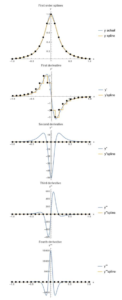
First Order Interpolation
The first order interpolation provides results for the first derivatives that are exactly similar to the results using forward finite difference. However, a first order interpolation function predicts zero second and higher derivatives. In the following tool, defines the interval at which the Runge function is sampled. The first derivative is calculated similar to the forward finite difference method. The higher derivatives are zero. The tool overlays the actual derivative with that predicted using the interpolation function. The black dots provide the values of the derivatives at the sampled points.
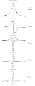
Second Order Interpolation
The second order interpolation provides much better results for  compared with the finite difference formulas. However, the third and fourth derivatives are equal to zero. Change the value of to see its effect on the results.
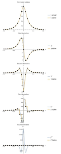
Third Order Interpolation
The third order interpolation (cubic splines) provides much better results for  compared with the finite difference formulas. However, the fourth derivative is equal to zero. Change the value of to see its effect on the results.
The following Mathematica code can be used to generate the tools above.
View Mathematica Codeh = 0.2;
n = 2/h + 1;
y = 1/(1 + 25 x^2);
yp = D[y, x];
ypp = D[yp, x];
yppp = D[ypp, x];
ypppp = D[yppp, x];
Data = Table[{-1 + h*(i - 1), (y /. x -> -1 + h*(i - 1))}, {i, 1, n}];
y2 = Interpolation[Data, Method -> "Spline", InterpolationOrder -> 1];
ypInter = D[y2[x], x];
yppInter = D[y2[x], {x, 2}];
ypppInter = D[y2[x], {x, 3}];
yppppInter = D[y2[x], {x, 4}];
Data1 = Table[{Data[[i, 1]], (ypInter /. x -> Data[[i, 1]])}, {i, 1, n}];
Data2 = Table[{Data[[i, 1]], (yppInter /. x -> Data[[i, 1]])}, {i, 1, n}];
Data3 = Table[{Data[[i, 1]], (ypppInter /. x -> Data[[i, 1]])}, {i, 1, n}];
Data4 = Table[{Data[[i, 1]], (yppppInter /. x -> Data[[i, 1]])}, {i, 1, n}];
a0 = Plot[{y, y2[x]}, {x, -1, 1}, Epilog -> {PointSize[Large], Point[Data]}, AxesLabel -> {"x", "y"}, BaseStyle -> Bold, ImageSize -> Medium, PlotRange -> All, PlotLegends -> {"y actual", "y spline"}, PlotLabel -> "First order splines"];
a1 = Plot[{yp, ypInter}, {x, -1, 1}, Epilog -> {PointSize[Large], Point[Data1]}, AxesLabel -> {"x", "y'"}, BaseStyle -> Bold, ImageSize -> Medium, PlotRange -> All, PlotLegends -> {"y'", "y'spline"}, PlotLabel -> "First derivative"];
a2 = Plot[{ypp, yppInter}, {x, -1, 1}, Epilog -> {PointSize[Large], Point[Data2]}, AxesLabel -> {"x", "y''"}, BaseStyle -> Bold, ImageSize -> Medium, PlotRange -> All, PlotLegends -> {"y''", "y''spline"}, PlotLabel -> "Second derivative"];
a3 = Plot[{yppp, ypppInter}, {x, -1, 1}, Epilog -> {PointSize[Large], Point[Data3]}, AxesLabel -> {"x", "y''"}, BaseStyle -> Bold, ImageSize -> Medium, PlotRange -> All, PlotLegends -> {"y'''", "y'''spline"}, PlotLabel -> "Third derivative"];
a4 = Plot[{ypppp, yppppInter}, {x, -1, 1}, Epilog -> {PointSize[Large], Point[Data4]}, AxesLabel -> {"x", "y''"}, BaseStyle -> Bold, ImageSize -> Medium, PlotRange -> All, PlotLegends -> {"y''''", "y''''spline"}, PlotLabel -> "Fourth derivative"];
Grid[{{a0}, {a1}, {a2}, {a3}, {a4}}]
import numpy as np
import sympy as sp
import matplotlib.pyplot as plt
from scipy.interpolate import UnivariateSpline
# UnivariateSpline used here for its derivative function is similar to Interp1d

x = sp.symbols('x')
x_val = np.arange(-1, 1,0.01)
h = 0.2
n = int(2/h + 1)
y = 1/(1 + 25*x**2)
yp = y.diff(x, n=1)
ypp = yp.diff(x, n=2)
yppp = ypp.diff(x, n=3)
ypppp = yppp.diff(x, n=4)
Data = [[-1 + h*i, (y.subs(x, -1 + h*i))] for i in range(n)]

y2 = UnivariateSpline([point[0] for point in Data],[point[1] for point in Data], k=1,s=0)
ypInter = y2.derivative(1)
try: yppInter = y2.derivative(2)
except Exception as e: print(e); yppInter = lambda x: 0;
try: ypppInter = y2.derivative(3)
except Exception as e: print(e); ypppInter = lambda x: 0;
try: yppppInter = y2.derivative(4)
except Exception as e: print(e); yppppInter = lambda x: 0;

Data1 = [[point[0], ypInter(point[0])] for point in Data]
Data2 = [[point[0], yppInter(point[0])] for point in Data]
Data3 = [[point[0], ypppInter(point[0])] for point in Data]
Data4 = [[point[0], yppppInter(point[0])] for point in Data]

plt.title("First order splines")
plt.xlabel("x"); plt.ylabel("y")
plt.scatter([point[0] for point in Data],[point[1] for point in Data], c='k')
plt.plot(x_val, [y.subs(x,i) for i in x_val], label="y actual")
plt.plot(x_val, [y2(i) for i in x_val], label="y spline")
plt.legend(); plt.grid(); plt.show()

plt.title("First derivative")
plt.xlabel("x"); plt.ylabel("y'")
plt.scatter([point[0] for point in Data1],[point[1] for point in Data1], c='k')
plt.plot(x_val, [yp.subs(x,i) for i in x_val], label="y'")
plt.plot(x_val, [ypInter(i) for i in x_val], label="y'spline")
plt.legend(); plt.grid(); plt.show()

plt.title("Second derivative")
plt.xlabel("x"); plt.ylabel("y''")
plt.scatter([point[0] for point in Data2],[point[1] for point in Data2], c='k')
plt.plot(x_val, [ypp.subs(x,i) for i in x_val], label="y''")
plt.plot(x_val, [yppInter(i) for i in x_val], label="y''spline")
plt.legend(); plt.grid(); plt.show()

plt.title("Third derivative")
plt.xlabel("x"); plt.ylabel("y'''")
plt.scatter([point[0] for point in Data3],[point[1] for point in Data3], c='k')
plt.plot(x_val, [yppp.subs(x,i) for i in x_val], label="y'''")
plt.plot(x_val, [ypppInter(i) for i in x_val], label="y'''spline")
plt.legend(); plt.grid(); plt.show()

plt.title("Fourth derivative")
plt.xlabel("x"); plt.ylabel("y''''")
plt.scatter([point[0] for point in Data4],[point[1] for point in Data4], c='k')
plt.plot(x_val, [ypppp.subs(x,i) for i in x_val], label="y''''")
plt.plot(x_val, [yppppInter(i) for i in x_val], label="y''''spline")
plt.legend(); plt.grid(); plt.show()