Engineering at Alberta Courses » Examples and Problems

Errors: Examples and Problems

Examples

Example 1

The width of a concrete beam is 250mm and the length is 10m. A length measurement device measured the width at 247mm while the length was measured at 9,997mm. Find the error and the relative error in each case.

Solution

For the width of the beam, the error is:

$E=250-247=3 mm$

The relative error is:

$E_r=\frac{3}{250} = 0.012 = 1.2\%$

For the length of the beam, the error is:

$E=10000-9997=3 mm$

The relative error is:

$E_r=\frac{3}{10000} = 0.0003 = 0.03\%$

This example illustrates that the value of the error itself might not give a good indication of how accurate the measurement is. The relative error is a better measure as it is normalized with respect to the actual value. It should be noted however, that sometimes the relative error is not a very good measure of accuracy. For example, if the true value is very close to zero, then the relative error might be a number that is approximately equal to $\frac{0}{0}$ and so it can give very unpredictable values. In that case, the error $E$ might be a better measure of error.

Example 2

Use the Babylonian method to find the square roots of 23.67 and 19532. For each case use an initial estimate of 1. Use a stopping criterion of $\varepsilon_s=0.1\%$ . Report the answer

to 4 significant digits.
to 4 decimal places.

Solution

The following table shows the Babylonian-method iterations to find the square root of 23.67 until $\varepsilon_r<0.001$ . Excel was used to produce the table. The criterion for stoppage was achieved after 6 iterations. table1
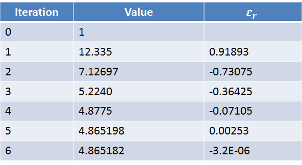
Therefore, the square root of 23.67 to 4 significant digits is 4.865. The square root of 23.67 to 4 decimal places is 4.8652.

The following table shows the Babylonian-method iterations to find the square root of 19532 until $\varepsilon_r<0.001$ . Excel was used to produce the table. The criterion for stoppage was achieved after 11 iterations. 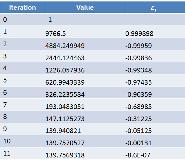Table2
Therefore, the square root of 19532 to 4 significant digits is 139.8. The square root of 19532 to 4 decimal places is 139.7569.

You can use Mathematica to show the square root of these numbers up to as many digits as you want. Notice that we used a fraction to represent 23.67, otherwise, it would resort to machine precision which could be less than the number of digits specified. Copy and paste the following code into your Mathematica to see the results:

View Mathematica Code:

t1=N[Sqrt[2367/100],200]
t3 = N[Sqrt[19532], 200]

View Python Code

import math
import sympy as sp
t1 = sp.N(math.sqrt(2367/100),200)
t3 = sp.N(math.sqrt(19532), 200)
print("t1:",t1)
print("t3:",t3)

The Babylonian method to find the square root of a number can also be coded in MATLAB. You can download the MATLAB file below:

Download Matlab File

Example 3

The $\cos(x)$ function where $x$ is in radian can be represented as the infinite series:

$\cos(x)=1-\frac{x^2}{2!}+\frac{x^4}{4!}-\cdots=\sum_{n=0}^{\infty}\frac{(-1)^n}{(2n)!}x^{2n}$

Let $i$ be the number of terms used to approximate the function $\cos(x)$ . Draw the curve showing the relative approximate error as a function of the number of terms used when approximating $\cos(1.5)$ and $\cos(10)$ . Also, draw the curve showing the value of the approximation in each case as a function of $i$ .

Solution

We are going to use the Mathematica software to produce the plot. First, a function will be created that is a function of the value of $x$ and the number of terms $i$ . This function has the form:

$ApproxCos(x,i)=\sum_{n=0}^{i-1}\frac{(-1)^n}{(2n)!}x^{2n}$

For example,

$ApproxCos(x,1)=1 \qquad ApproxCos(x,2)=1-\frac{x^2}{2!} \qquad ApproxCos(x,3)=1-\frac{x^2}{2!}+\frac{x^4}{4!}$

The relative approximate error when using $i$ terms can be calculated as follows:

$\varepsilon_r=\frac{ApproxCos(x,i)-ApproxCos(x,i-1)}{ApproxCos(x,i)}$

A table of the relative error for $i$ between 2 and 20 can then be generated. Finally, the list of relative errors and the approximations can be plotted using Mathematica.
Note the following in the code. The best way to achieve good accuracy is to define the approximation function with arbitrary precision. Therefore, no decimal points should be used. Otherwise, machine precision would be used and might lead to deviation from the accurate solution as will be shown in the next example. The angles are defined using fractions and after evaluating the functions, the numerical evaluation function N[] is used to numerically evaluate the approximate value after adding enough terms!

View Mathematica Code

ApproxCos[x_, i_] := Sum[(-1)^n*x^(2 n)/((2 n)!), {n, 0, i - 1}]
Angle1 = 15/10;
Angle2 = 10;
ertable1 = Table[{i, N[(ApproxCos[Angle1, i] - ApproxCos[Angle1, i - 1])/ApproxCos[Angle1, i]]}, {i, 2, 20}]
ertable2 = Table[{i, N[(ApproxCos[Angle2, i] - ApproxCos[Angle2, i - 1])/ApproxCos[Angle2, i]]}, {i, 2, 20}]
ListPlot[{ertable1, ertable2}, PlotRange -> All, Joined -> True, AxesLabel -> {"i", "relative error"}, AxesOrigin -> {0, 0}, PlotLegends -> {"Relative error in Cos(1.5)", "Relative error in Cos(10)"}]
cos1table = Table[{i, N[ApproxCos[Angle1, i]]}, {i, 2, 20}]
cos2table = Table[{i, N[ApproxCos[Angle2, i]]}, {i, 2, 20}]
ListPlot[{cos1table, cos2table}, Joined -> True,  AxesLabel -> {"i", "Cos approximation"}, AxesOrigin -> {0, 0},  PlotLegends -> {"Cos(1.5) approximation", "Cos(10) approximation"}, PlotRange -> {{0, 20}, {-10, 10}}]
N[ApproxCos[Angle1, 20]]
N[ApproxCos[Angle2, 20]]

View Python Code

import math
import sympy as sp
import matplotlib.pyplot as plt

def ApproxCos(x,i):
  return sum([(-1)**n * x**(2*n)/math.factorial(2*n) for n in range(i)])
Angle1 = 15/10
Angle2 = 10
ertable1 = [(ApproxCos(Angle1, i) - ApproxCos(Angle1, i - 1))/ApproxCos(Angle1, i) for i in range(2,20)]
print("ertable1:",ertable1)
ertable2 = [(ApproxCos(Angle2, i) - ApproxCos(Angle2, i - 1))/ApproxCos(Angle2, i) for i in range(2,20)]
print("ertable2:",ertable2)

i = [i for i in range(2,20)]

plt.plot(i, ertable1, label="Relative error in Cos(1.5)")
plt.plot(i, ertable2, label="Relative error in Cos(10)")
plt.ylabel('Relative Error'); plt.xlabel('i')
plt.legend(); plt.grid(); plt.show()

cos1table = [ApproxCos(Angle1, i) for i in range(2, 20)] 
cos2table = [ApproxCos(Angle2, i) for i in range(2, 20)]
print("cos1table:",cos1table)
print("cos2table:",cos2table)

plt.plot(i, cos1table, label="Cos(1.5) approximation")
plt.plot(i, cos2table, label="Cos(10) approximation")
plt.ylabel('Cos Approximation'); plt.xlabel('i')
plt.xlim(0,20); plt.ylim(-10,10)
plt.legend(); plt.grid(); plt.show()

print("ApproxCos(Angle1, 20):",ApproxCos(Angle1, 20))
print("ApproxCos(Angle2, 20):",ApproxCos(Angle2, 20))

Approximate the function cos(x) with a specified number of terms is coded in MATLAB as follows. The main script calls the function approxcos prepared in another file and outputs the approximation.

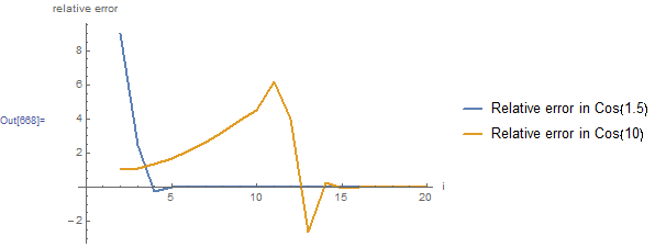
Download MATLAB file for the main script

Download MATLAB file for the example function

The plot of the relative error is shown below. For $\cos(1.5)$ , the relative error decreases dramatically and is already very close to zero when 4 terms are used! However, for $\cos(10)$ , the relative error starts approaching zero when 14 terms are used!
Plot1
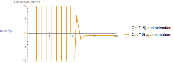
The plot of the approximate values of $\cos(1.5)$ and $\cos(10)$ as a function of the number of terms is shown below. The approximation for $\cos(1.5)$ approaches its stabilized and accurate value of 0.0707372 using only 3 terms. However, the approximation for $\cos(10)$ keeps oscillating taking very high positive values followed by very high negative values as a function of $i$ . The approximation starts approaching its stabilized and accurate value of around -0.83907 after using 14 terms!
Plot2

Example 4

The $\cos(x)$ function where $x$ is in radian can be represented as the infinite series:

$\cos(x)=1-\frac{x^2}{2!}+\frac{x^4}{4!}-\cdots=\sum_{n=0}^{\infty}\frac{(-1)^n}{(2n)!}x^{2n}$

Let $i$ be the number of terms used to approximate the function $\cos(x)$ . Show the difference between using machine precision and arbitrary precision in Mathematica in the evaluation of $\cos(100)$ .

Solution

Each positive term in the infinite series of $\cos(x)$ is followed by a negative term. In addition, each term has a value of $\frac{x^{2n}}{(2n)!}$ . For $x=100$ , the series would be composed of adding and subtracting very large numbers. If machine precision is used, then round-off errors will lead to the inability of the series to actually converge to the correct solution. The code below shows that using 140 terms, the series gives the value of 0.862314 which is a very accurate representation of $\cos(100)$ . This value is obtained by first evaluating the sum using arbitrary precision and then numerically evaluating the result using machine precision. If, on the other hand, we use a machine precision for the angle, the computations are done in machine precision. In this case, the series converges, however, to the value of $2.64917\times 10^{26}$ ! This is because in effect we are adding and subtracting very large numbers, each with a small round-off error because of using machine precision. This problem is termed Loss of Significance. Since the true value is much smaller than the individual terms, then, the accuracy of the calculation relies on the accuracy of the differences between the terms. If only a certain number of significant digits is retained, then, subtracting each two large terms leads to loss of significance!

View Mathematica Code

ApproxCos[x_, i_] := Sum[(-1)^n*x^(2 n)/((2 n)!), {n, 0, i - 1}]
N[ApproxCos[100, 140]]
ApproxCos[N[100], 140]
ApproxCos[N[100], 300]
Cos[100.]

View Python Code

import math
import numpy as np
import sympy as sp
def ApproxCos(x,i):
  return sum([(-1)**n * x**(2*n)/sp.Float(math.factorial(2*n),100) for n in range(i)])
print("N(ApproxCos(100, 140)):",sp.N(ApproxCos(100, 140)))
print("ApproxCos(N(100), 140):",ApproxCos(sp.N(100), 140))
print("ApproxCos(N(100), 300):",ApproxCos(sp.N(100), 300))
print("Cos(100):",np.cos(100))

Problems

Use the Babylonian method to find the square root of your ID number. Use an initial estimate of 1. Use a stopping criterion of $\varepsilon_s=0.1\%$ . Report the answer in two formats: 1) approximated to 4 significant digits, and 2) to 4 decimal places.
Find two examples of random errors and two examples of systematic errors.
Find a calculating device (your cell phone calculator) and describe what happens when you divide 1 by 3 and then multiply the result by 3. Repeat the calculation by dividing 1 by 3, then divide the result by 7. Then, take the result and multiply it by 3, then multiply it by 7. Can you infer how your cell phone calculator stores numbers?
Using the infinite series representation of the $\sin$ function to approximate $\sin(1)$ and $\sin(10)$ , draw the curve showing the relative approximate error as a function of the number of terms used for each.
Using Machine Precision in Mathematica, find a number $x$ that satisfies:
$N[1+0.5x]-1=0$ while $N[1+x]-1=x$ . Compare that number with MachineEpsilon in Mathematica