
Polynomial Interpolation: Newton Interpolating Polynomials
Newton Interpolating Polynomials
As stated in the introduction, the matrix formed in Equation 1 can be ill-conditioned and difficult to find an inverse for. A simpler method can be used to find the interpolating polynomial using Newton’s Interpolating Polynomials formula for fitting a polynomial of degree  through
  data points
  with
with  :
:
![\[ f_n(x)=b_1+b_2(x-x_1)+b_3(x-x_1)(x-x_2)+\cdots+b_{n+1}(x-x_1)(x-x_2)\cdots(x-x_n) \]](https://engcourses-uofa.ca/wp-content/ql-cache/quicklatex.com-68440c188f4ed3e251f5a1c7d4bd02ae_l3.png "Rendered by QuickLaTeX.com")
where the coefficients  are defined recursively using the divided differences as follows:
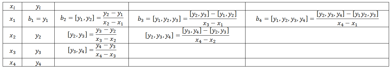
![\[\begin{split} b_1&=y_1\\ b_2&=[y_1,y_2]=\frac{y_2-y_1}{x_2-x_1}\\ b_3&=[y_1,y_2,y_3]=\frac{[y_2,y_3]-[y_1,y_2]}{x_3-x_1}=\frac{\frac{y_3-y_2}{x_3-x_2}-\frac{y_2-y_1}{x_2-x_1}}{x_3-x_1}\\ \vdots &\\ b_{n+1}&=[y_1,y_2,y_3,\cdots,y_{n+1}]=\frac{[y_2,y_3,\cdots,y_{n+1}]-[y_1,y_2,y_3,\cdots,y_{n}]}{x_{n+1}-x_1} \end{split} \]](https://engcourses-uofa.ca/wp-content/ql-cache/quicklatex.com-49413b6651e0e40147b1cf17f2d55841_l3.png "Rendered by QuickLaTeX.com")
This recursive divided differences are illustrated in the following table:
The following Mathematica code implements a recursive function “f” that produces the coefficients .
Data = {{1, 3}, {4, 5}, {5, 6}, {6, 8}, {7, 8}};
f[anydata_] := If[Length[anydata] == 1, anydata[[1, 2]], If[Length[anydata] ==2, (anydata[[2, 2]] - anydata[[1, 2]])/(anydata[[2, 1]] -anydata[[1, 1]]), (f[Drop[anydata, 1]] - f[Drop[anydata, -1]])/(anydata[[Length[anydata], 1]] - anydata[[1, 1]])]]
NP[anydata_] := Sum[f[anydata[[1 ;; i]]]*Product[(x - anydata[[j, 1]]), {j, 1, i - 1}], {i, 1, Length[anydata]}]
(*Using the Newton polynomial function*)
y = Expand[NP[Data]]
(*Using the interpolating polynomial built-in function*)
y2 = Expand[InterpolatingPolynomial[Data, x]]
import numpy as np
import sympy as sp
sp.init_printing(use_latex=True)

Data = [(1, 3), (4, 5), (5, 6), (6, 8), (7, 8)]
x = sp.symbols('x')
def f(anydata):
  if len(anydata) == 1:
    return anydata[0][1]
  elif len(anydata) == 2:
    return (anydata[1][1] - anydata[0][1])/(anydata[1][0] -anydata[0][0])
  else:
    return (f(anydata[1:]) - f(anydata[:-1]))/(anydata[len(anydata)-1][0] - anydata[0][0])
def NP(anydata):
  return sum([f(anydata[0:i+1])*np.prod([(x - anydata[j][0]) for j in range(i)]) for i in range(len(anydata))])
# Using the Newton polynomial function
display("y: ",sp.expand(NP(Data)))
# Using the interpolating polynomial built-in function
display("y2: ",sp.interpolate(Data, x))
Newton’s formula for generating an interpolating polynomial adopts a form similar to that of a Taylor’s polynomial but is based on finite differences rather than the derivatives. I.e., the coefficients are calculated using finite difference. One advantage to this form is that the degree of a Newton’s interpolating polynomial can be increased (or decreased) automatically by adding (or removing) more terms corresponding to new points without discarding existing terms.
Example 1
Using Newton’s interpolating polynomials, find the interpolating polynomial to the data: (1,1),(2,5).
Solution
We have two data points, so, we will create a polynomial of the first degree. Therefore:
![\[ b_1=y_1=1\qquad b_2=\frac{5-1}{2-1}=4 \]](https://engcourses-uofa.ca/wp-content/ql-cache/quicklatex.com-46b71e9109599c501be0012c0c1ea7a7_l3.png "Rendered by QuickLaTeX.com")
Therefore, the interpolating polynomial has the form:
![\[ y=1+4(x-1)=1+4x-4=-3+4x \]](https://engcourses-uofa.ca/wp-content/ql-cache/quicklatex.com-389fcac9e9f9eb5a3f52731463060a27_l3.png "Rendered by QuickLaTeX.com")
Example 2
Using Newton’s interpolating polynomials, find the interpolating polynomial to the data: (1,1),(2,5),(3,2).
Solution
We have three data points, so, we will create a polynomial of the second degree. Therefore:
![\[ b_1=y_1=1\qquad b_2=\frac{5-1}{2-1}=4 \qquad b_3=\frac{\frac{2-5}{3-2}-\frac{5-1}{2-1}}{3-1}=-3.5 \]](https://engcourses-uofa.ca/wp-content/ql-cache/quicklatex.com-6f8535cbef6d0207e01fd453bc945a3c_l3.png "Rendered by QuickLaTeX.com")
Therefore, the interpolating polynomial has the form:
![\[ y=1+4(x-1)-3.5(x-1)(x-2)=-3.5x^2+14.5x-10 \]](https://engcourses-uofa.ca/wp-content/ql-cache/quicklatex.com-aa0844431a26b7ca2b649ed2d1f1ce57_l3.png "Rendered by QuickLaTeX.com")
Example 3
Using Newton’s interpolating polynomials, find the interpolating polynomial to the data: (1,1),(2,5),(3,2),(3.2,7),(3.9,4).
Solution
The divided difference table for these data points were created in excel as follows:
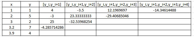
Therefore, the Newton’s Interpolating Polynomial has the form:
![\[\begin{split} y=&1+4(x-1)-3.5(x-1)(x-2)+12.19697(x-1)(x-2)(x-3)\\ &-14.346144(x-1)(x-2)(x-3)(x-3.2)\\ =&-14.3461x^4+144.181x^3-509.935x^2+739.728x-358.628 \end{split} \]](https://engcourses-uofa.ca/wp-content/ql-cache/quicklatex.com-4a31ba4a94d14fac179a9dfcecc645c1_l3.png "Rendered by QuickLaTeX.com")
Hi! I just want to let you know that the matlab code attached doesn’t seem to work for me as matlab keeps on saying that ddiff function is not found and suggests me to use diff instead. However, using diff results in “Unable to perform assignment because the indices on the
left side are not compatible with the size of the right side.”
I have added a link to download the ddif function.