Engineering at Alberta Courses

Numerical Integration: Trapezoidal Rule

Trapezoidal Rule

Let $f:[a,b]\rightarrow \mathbb{R}$ . By dividing the interval $[a,b]$ into many subintervals, the trapezoidal rule approximates the area under the curve by linearly interpolating between the values of the function at the junctions of the subintervals, and thus, on each subinterval, the area to be calculated has a shape of a trapezoid. For simplicity, the width of the trapezoids is chosen to be constant. Let $n$ be the number of intervals with $a=x_0 < x_1 < x_2 < \cdots < x_n=b$ and constant spacing $h=x_{i+1}-x_i$ . The trapezoidal method can be implemented as follows:

$I_T=\int_{a}^b\!f(x)\,\mathrm{d}x\approx \frac{h}{2}\sum_{i=1}^{n}\left(f(x_{i-1})+f(x_i)\right)=\frac{h}{2}(f(x_0)+2f(x_1)+2f(x_2)+\cdots+2f(x_{n-1})+f(x_n))$

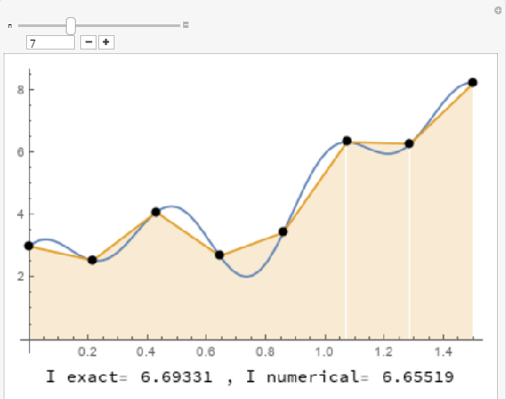
The following tool illustrates the implementation of the trapezoidal rule for integrating the function $f:[0,1.5]\rightarrow \mathbb{R}$ defined as:

$f(x)= 2 + 2 x + x^2 + \sin{(2 \pi x)} + \cos{(2 \pi \frac{x}{0.5})}$

Use the slider to see the effect of increasing the number of intervals on the approximation.

The following Mathematica code can be used to numerically integrate any function $f$ on the interval $[a,b]$ using the trapezoidal rule.

View Mathematica Code

IT[f_, a_, b_, n_] := (h = (b - a)/n; Sum[(f[a + (i - 1)*h] + f[a + i*h])*h/2, {i, 1, n}])
f[x_] := 2 + 2 x + x^2 + Sin[2 Pi*x] + Cos[2 Pi*x/0.5];
IT[f, 0, 1.5, 1.0]
IT[f, 0, 1.5, 18.0]

View Python Code

import numpy as np 
def IT(f, a, b, n):
  h = (b - a)/n
  return sum([(f(a + i*h) + f(a + (i + 1)*h))*h/2 for i in range(int(n))])
def f(x): return 2 + 2*x + x**2 + np.sin(2*np.pi*x) + np.cos(2*np.pi*x/0.5)
print(IT(f, 0, 1.5, 1.0))
print(IT(f, 0, 1.5, 18.0))

The following link provides the MATLAB codes for implementing the trapezoidal rule.

MATLAB files: File 1 (trap.m)

Error Analysis

An extension of Taylor’s theorem can be used to find how the error changes as the step size $h$ decreases. Given a function $f$ and its interpolating polynomial of degree $n$ ( $p_n(x)$ ), the error term between the interpolating polynomial and the function is given by (See the Mathematical Background section for a proof):

$f(x)=p_n(x)+\frac{f^{n+1}(\xi)}{(n+1)!}\prod_{i=1}^{n+1}(x-x_{i})$

Where $\xi$ is in the domain of the function $f$ and is dependent on the point $x$ . The error in the calculation of trapezoidal number $i$ between the points $x_{i-1}$ and $x_{i}$ will be estimated based on the above formula assuming a linear interpolation between the points $x_{i-1}$ and $x_i$ . Therefore:

$\begin{split}|E_i|&=\left|\int_{x_{i-1}}^{x_i}\! f(x)-p_1(x)\,\mathrm{d}x\right|=\left|\int_{x_{i-1}}^{x_i}\!\frac{f''(\xi)}{2}(x-x_{i-1})(x-x_i)\,\mathrm{d}x\right|\\&\leq \max_{\xi\in[x_{i-1},x_i]}\frac{|f''(\xi)|h^3}{12}\end{split}$

If $n$ is the number of subdivisions (number of trapezoids), i.e., $nh=b-a$ , then:

$|E|=|nE_i|\leq \max_{\xi\in[a,b]}\frac{|f''(\xi)|nh^3}{12}=\max_{\xi\in[a,b]}\frac{|f''(\xi)|(b-a)h^2}{12}$

In the above error analysis, we disregarded higher order terms than $f''$ . Although this simplified the calculations and sufficed our purpose, here we demonstrate a general error analysis containing higher order terms. We will use the results later in explaining the Romberg’s Method.

Consider a continuous function $f(x)$ defined on an interval $[a,b]$ . If the interval is discretized into $n$ sub intervals $[x_i,x_{i+1}]$ such that $a=x_0<x_1<\cdots<x_n=b$ , the trapezoidal rule estimates the integration of $f(x)$ over a sub interval $[x_i, x_{i+1}]$ as:

$\int_{x_i}^{x_{i+1}} f(x)\mathrm d x\approx \frac{h_i}{2}\left( f(x_i) + f(x_{i+1})\right)$

where $h_i = x_{i+1}-x_{i}$

To find the order of error of the above estimation, we should find the terms represented by $\mathcal O(h_i^k)$ in:

(I) $\int_{x_i}^{x_{i+1}} f(x)\mathrm d x= \frac{h_i}{2}\left( f(x_i) + f(x_{i+1})\right) + \mathcal O(h_i^k)$

where $k$ in the order of accuracy (to be determined).

To this end, we first consider writing $f(x)$ for $x\in [x_i, x_{i+1}]$ by its the Taylor series expansion about $y_i=\frac{x_i + x_{i+1}}{2}$ being is the midpoint of the interval $[x_i, x_{i+1}]$ . Therefore, substituting the Taylor series expansion into $\int_{x_i}^{x_{i+1}} f(x)\mathrm d x$ leads to,

$\begin{split}\int_{x_i}^{x_{i+1}} f(x)\mathrm d x&=\int_{x_i}^{x_{i+1}} \left( f(y_i)+(x-y_i)f'(y_i)+\frac{1}{2}(x-y_i)^2f''(y_i)+\frac{1}{6}(x-y_i)^3f'''(y_i)+\dots \right)\mathrm d x\\&=h_if(y_i)+\frac{1}{2}(x-y_i)^2\Big |_{x_i}^{x_{i+1}}f'(y_i)+\frac{1}{6}(x-y_i)^3 \Big |_{x_i}^{x_{i+1}}f''(y_i)\\ &+\frac{1}{24}(x-y_i)^4 \Big |_{x_i}^{x_{i+1}}f''(y_i)+\cdots\end{split}$

which is eventually evaluated as,

(II) $\int_{x_i}^{x_{i+1}} f(x)\mathrm d x= h_if(y_i)+\frac{1}{24}h_i^3f''(y_i)+\frac{1}{1920}h_i^5f^{(4)}(y_i)+\cdots$

Leaving this result for now and getting back to the trapezoidal rule, we can write $\frac{f(x_i)+f(x_{i+1})}{2}$ using its Taylor series expansion as follows.

If the Taylor series expansions for $f(x_i)$ and $f(x_{i+1})$ are written as,

$\begin{split}f(x_i)&=f(y_i)-\frac{1}{2}h_if'(y_i)+\frac{1}{8}h^2_if''(y_i)-\frac{1}{48}h^3_if'''(y_i)+\cdots\\f(x_{i+1})&=f(y_i)+\frac{1}{2}h_if'(y_i)+\frac{1}{8}h^2_if''(y_i)+\frac{1}{48}h^3_if'''(y_i)+\cdots\end{split}$

therefore,

$\frac{f(x_i)+f(x_{i+1})}{2}=f(y_i)+\frac{1}{8}h^2_if''(y_i)+\frac{1}{384}h^4_if^{(4)}(y_i)+ \cdots$

Note that the derivatives of odd order, i.e. $f', f''', f^{(5)}, \dots$ vanish.

Solving the above equation for $f(y_i)$ and substituting the resultant expression into the right-hand side of Eq. II, leads to,

$\int_{x_i}^{x_{i+1}} f(x)\mathrm d x= h_i\frac{f(x_i)+f(x_{i+1})}{2}-\frac{1}{12}h_i^3f''(y_i)-\frac{1}{480}h_i^5f^{(4)}(y_i)+\cdots$

Comparing this result with Eq. I, we can say that the trapezoidal rule is third-order accurate over a sub-interval, in other words,

(I) $\int_{x_i}^{x_{i+1}} f(x)\mathrm d x= \frac{h_i}{2}\left( f(x_i) + f(x_{i+1})\right) + \mathcal O(h_i^3)$

We should now proceed to analyze the error of the trapezoidal rule over the entire interval $[a,b]$ . If we consider a similar length, $h$ , for each sub interval $[x_i, x_{i+1}]$ of $[a,b]$ discretized as $a=x_0< x_1<\cdots <x_n=b$ , we can write,

$\begin{split}\int_a^b f(x)\mathrm dx = \sum_{i=0}^{n-1}\int_{x_i}^{x_{i+1}}f(x)\mathrm dx &= \frac{h}{2}\Big ( f(a) + f(b) +2\sum_{j=1}^{n-1} f(x_j)\Big )\\ & - \frac{h^3}{12}\sum_{i=0}^{n-1}f''(y_i)- \frac{h^5}{480}\sum_{i=0}^{n-1}f^{(4)}(y_i) + \cdots\end{split}$

The summations of terms of derivatives can be replaced with their values determined using the intermediate value theorem. The intermediate value theorem states that if a function $g(x)$ is continuous over the interval $[a_1,a_2]$ , there is $c\in[a_1,a_2]$ such that $g(s)=s$ for any $s$ falling within the values of $g(a_1)$ and $g(a_2)$ .

Therefore, for the continuous function $f''(x)$ over $[a,b]$ , if we set $a_1$ and $a_2$ within $[a,b]$ such that $f''(a_1)=\underset{x\in [a,b]}{\min} f''(y)$ and $f''(a_2)=\underset{x\in [a,b]}{\max} f''(y)$ , we can write,

$f''(a_1)\le \frac{\sum_{i=0}^{n-1}f''(y_i)}{n}\le f''(a_2)$

meaning that there is a number $\xi\in [a,b]$ such that $f''(\xi)= \frac{\sum_{i=0}^{n-1}f''(y_i)}{n}$ . Consequently,

$\sum_{i=0}^{n-1}f''(y_i)= n f''(\xi)$

With the same method, we can write $\sum_{i=0}^{n-1}f^{(4)}(y_i)$ as,

$\sum_{i=0}^{n-1}f^{(4)}(y_i)= n f^{(4)}(\eta)$

for $\eta\in [a,b]$ .

Using the above values of the summations we get,

$\begin{split}\int_a^b f(x)\mathrm dx = \sum_{i=0}^{n-1}\int_{x_i}^{x_{i+1}}f(x)\mathrm dx &= \frac{h}{2}\Big ( f(a) + f(b) +2\sum_{j=1}^{n-1} f(x_j)\Big )\\ & - \frac{h^3}{12}nf''(\xi)- \frac{h^5}{480}nf^{(4)}(\eta) + \cdots\end{split}$

As $n=\frac{b-a}{h}$ , we can conclude that

$\begin{split}\int_a^b f(x)\mathrm dx &=\frac{h}{2}\Big ( f(a) + f(b) +2\sum_{j=1}^{n-1} f(x_j)\Big )\\ & - (b-a)\frac{h^2}{12}f''(\xi)- (b-a)\frac{h^4}{480}f^{(4)}(\eta) + \cdots\end{split}$

Indicating that the trapezoidal rule for integration of $f(x)$ over any interval $[a,b]$ is second-order accurate.

Example

Using the trapezoidal rule with $n=4$ , calculate $I_T$ and compare with the exact integral of the function $f(x)=e^x$ on the interval $[0,2]$ . Find the value of $h$ so that the error is less than 0.001.

Solution

Since $n=4$ the spacing $h$ can be calculated as:

$h=\frac{b-a}{n}=\frac{2-0}{4}=0.5$

Therefore, $x_0=0$ , $x_1=0.5$ , $x_2=1$ , $x_3=1.5$ , and $x_4=2.0$ . The values of the function at these points are given by:

$f(x_0)=e^0=1.00\qquad f(x_1)=e^{0.5}=1.6487 \qquad f(x_2)=e^{1}=2.7183$

$f(x_3)=e^{1.5}=4.4817 \qquad f(x_4)=e^{2}=7.3891$

According to the trapezoidal rule we have:

$\begin{split}I_T&=\frac{h}{2}(f(x_0)+2f(x_1)+2f(x_2)+\cdots+2f(x_{n-1})+f(x_n))\\&=\frac{0.5}{2} (1 + 2\times 1.6487 + 2\times 2.7183 + 2\times 4.4817 + 7.3891) = 6.522\end{split}$

Which is already a very good approximation to the exact value of $I=6.38906$ even though only 4 intervals were used.

Error Bounds

The total error obtained when $h=0.5$ is indeed less than the error bounds obtained by the formula listed above. For $I_T$ , the error in the estimation is bounded by:

$|E|\leq \max_{\xi\in[a,b]}|f''(\xi)| (b-a)\frac{h^2}{12}=e^{2}(2-0)\frac{0.25}{12}=0.3079$

The error $|I-I_T|=|6.38906-6.522|=0.13294$ is indeed less than that upper bound. The same formula can be used to find the value of $h$ so that the error is bounded by 0.001:

$e^{2}(2-0)\frac{h^2}{12}=0.001\Rightarrow h=0.0285$

Therefore, to guarantee an error less than 0.001 using $I_T$ , the interval will have to be divided into: $\frac{2}{0.0285}=70.175$ parts. Therefore, at least 71 trapezoids are needed! In this case, $I_T=6.38948$ and $|E|=|6.38948-6.38906|=0.00042$ .

Open Educational Resources