Engineering at Alberta Courses » Nonlinear Regression

Curve Fitting: Nonlinear Regression

Nonlinear Regression

In nonlinear regression, the model function $y$ is a nonlinear function of $x$ and of the parameters $a_1, a_2,\cdots,a_m$ . Given a set of $n$ data points $(x_i,y_i)$ with $1\leq i \leq n$ , curve fitting starts by assuming a model $y(x)$ with $m$ parameters. The parameters can be obtained by minimizing the least squares:

$S=\sum_{i=1}^n (y(x_i)-y_i)^2$

In order to find the parameters of the model that would minimize $S$ , $m$ equations of the following form are solved:

$\frac{\partial S}{\partial a_k}=\sum_{i=1}^n\left(2\left(y(x_i)-y_i\right)\frac{\partial y}{\partial a_k}\bigg|_{x=x_i}\right)=0$

Since $y(x)$ is nonlinear in the coefficients, the $m$ equations formed are also nonlinear and can only be solved using a nonlinear equation solver method such as the Newton Raphson method described before. We are going to rely on the built-in NonlinearModelFit function in Mathematica that does the required calculations.

Example 1

The following data describes the yield strength $\sigma_y$ and the plastic strain $\varepsilon_p$ obtained from uniaxial experiments where the first variable is the plastic strain and the second variable is the corresponding yield strength: (0.0001,204.18),(0.0003,226.4),(0.0015,270.35),(0.0025,276.86),(0.004,296.86),(0.005,299.3),(0.015,334.65),(0.025,346.56),(0.04,371.81),(0.05,377.45),(0.1,398.01),(0.15,422.45),(0.2,434.42).
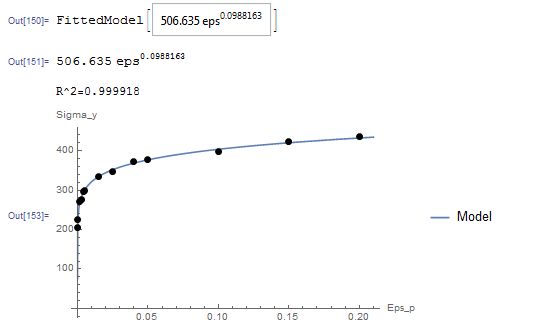
Use the NonlinearModelFit function in Mathematica to find the best fit for the data assuming the relationship follows the form:

$\sigma_y=K\varepsilon_p^n$

Solution

While this model can be linearized as described in the previous section, the NonlinearModelFit will be used. The array of data is input as a list in the variable Data. The NonlinearModelFit function is then used and the output is stored in the variable: “model”. The form of the best fit function is evaluated using the built-in function Normal[model]. $R^2$ can be evaluated as well as shown in the code below. The values of $K$ and $n$ that describe the best fit are $K=506.64$ and $n=0.0988$ . Therefore, the best-fit model is:

$\sigma_y=506.64\varepsilon_p^{0.0988}$

The following is the Mathematica code used along with the output
View Mathematica Code

Data = {{0.0001, 204.18}, {0.0003, 226.4}, {0.0015, 270.35}, {0.0025, 276.86}, {0.004, 296.86}, {0.005, 299.3}, {0.015, 334.65}, {0.025,346.56}, {0.04, 371.81}, {0.05, 377.45}, {0.1, 398.01}, {0.15, 422.45}, {0.2, 434.42}};
model = NonlinearModelFit[Data, Kk*eps^(n), {Kk, n}, eps]
y = Normal[model]
Print["R^2=",R2 = model["RSquared"]]
Plot[y, {eps, 0, 0.21}, Epilog -> {PointSize[Large], Point[Data]}, PlotLegends -> {"Model"}, AxesLabel -> {"Eps_p", "Sigma_y"}, AxesOrigin -> {0, 0}]

View Python Code

import numpy as np
import matplotlib.pyplot as plt
from scipy.optimize import curve_fit

Data = [[0.0001, 204.18], [0.0003, 226.4], [0.0015, 270.35], [0.0025, 276.86], [0.004, 296.86], [0.005, 299.3], [0.015, 334.65], [0.025,346.56], [0.04, 371.81], [0.05, 377.45], [0.1, 398.01], [0.15, 422.45], [0.2, 434.42]]
def f(eps, k, n): return k*eps**n
coeff, covariance = curve_fit(f, [point[0] for point in Data],
                                 [point[1] for point in Data])
print("coeff: ",coeff)
x_val = np.arange(0,0.21,0.001)
plt.title('%.5feps**(%.5f)' % tuple(coeff))
plt.plot(x_val, f(x_val, coeff[0], coeff[1]))
plt.scatter([point[0] for point in Data], [point[1] for point in Data], c='k')
plt.xlabel("Eps_p"); plt.ylabel("Sigma_y")
plt.grid(); plt.show()

# R squared
x = np.array([point[0] for point in Data])
y = np.array([point[1] for point in Data])
y_fit = f(x, coeff[0], coeff[1])
ss_res = np.sum((y - y_fit)**2)
ss_tot = np.sum((y - np.mean(y))**2)
r2 = 1 - (ss_res / ss_tot)
print("R Squared: ",r2)

nonlinearregres

The following links provide the MATLAB codes for implementing a nonlinear model fit for yield strength vs plastic strain. The function for the model is provided in File 2.

MATLAB files: File 1 (ex9_6.m) File 2 (plastic.m)

Example 2

Exponential and Logarithmic Models offer a wide range of model functions that can be used for various engineering applications. An example is the exponential model that describes an initial rapid increase in the dependent variable $y$ which then levels off to become asymptotic to an upper limit $a_1$ :

$y(x)=a_1(1-e^{-a_2x})$

where $a_1$ and $a_2$ are the model parameters. For plastic materials, Armstrong and Frederick proposed this model in 1966 (republished here in 2007) to describe how a quantity called the “Centre of the Yield Surface” changes with the increase in the plastic strain. If $\alpha$ is the centre of the yield surface and $\varepsilon_p$ is the plastic strain, then, the model for $\alpha$ has the form:

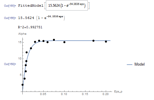
$\alpha = C\left(1-e^{-\gamma \varepsilon_p}\right)$

Find the values of $C$ and $\gamma$ for the best fit to the experimental data $({\varepsilon_p}_i,\alpha_i)$ given by: (0.0001,2.067),(0.005,3.96),(0.0075,6.22),(0.008,8.07),(0.009,9.32),(0.01,12.02),(0.02,13.2),(0.03,15.22),(0.04,15.51),(0.05,15.44),(0.06,15.1),(0.075,15.76),(0.1,15.11),(0.17,15.53),(0.2,15.26)

Solution

Unlike the model in the previous question, this model cannot be linearized. The NonlinearModelFit built-in function in Mathematica will be used. The array of data is input as a list in the variable Data. The NonlinearModelFit function is then used and the output is stored in the variable: “model”. The form of the best fit function is evaluated using the built-in function Normal[model]. $R^2$ can be evaluated as well as shown in the code below. The values of $C$ and $\gamma$ that describe the best fit are $C=15.5624$ and $\gamma=94.3836$ . Therefore, the best-fit model is:

$\alpha = 15.5624\left(1-e^{-94.3836 \varepsilon_p}\right)$

The following is the Mathematica code used along with the output

View Mathematica Code

Data = {{0.0001, 2.067}, {0.005, 3.96}, {0.0075, 6.22}, {0.008,8.07}, {0.009, 9.32}, {0.01, 12.02}, {0.02, 13.2}, {0.03,15.22}, {0.04, 15.51}, {0.05, 15.44}, {0.06, 15.1}, {0.075,15.76}, {0.1, 15.11}, {0.17, 15.53}, {0.2, 15.26}};
model = NonlinearModelFit[Data, Cc (1 - E^(-gamma*eps)), {Cc, gamma}, eps]
y = Normal[model]
Print["R^2=", R2 = model["RSquared"]]
Plot[y, {eps, 0, 0.21}, Epilog -> {PointSize[Large], Point[Data]}, PlotLegends -> {"Model"}, AxesLabel -> {"Eps_p", "Alpha"}, AxesOrigin -> {0, 0}]

View Python Code

import numpy as np
import matplotlib.pyplot as plt
from scipy.optimize import curve_fit

Data = [[0.0001, 2.067], [0.005, 3.96], [0.0075, 6.22], [0.008,8.07], [0.009, 9.32], [0.01, 12.02], [0.02, 13.2], [0.03,15.22], [0.04, 15.51], [0.05, 15.44], [0.06, 15.1], [0.075,15.76], [0.1, 15.11], [0.17, 15.53], [0.2, 15.26]]
def f(eps, c, gamma): return c*(1 - np.exp(-gamma*eps))
coeff, covariance = curve_fit(f, [point[0] for point in Data],
                                 [point[1] for point in Data])
print("coeff: ",coeff)
x_val = np.arange(0,0.21,0.001)
plt.title('%.5f(1 - e**(-%.5feps))' % tuple(coeff))
plt.plot(x_val, f(x_val, coeff[0], coeff[1]))
plt.scatter([point[0] for point in Data], [point[1] for point in Data], c='k')
plt.xlabel("Eps_p"); plt.ylabel("Alpha")
plt.grid(); plt.show()

# R squared
x = np.array([point[0] for point in Data])
y = np.array([point[1] for point in Data])
y_fit = f(x, coeff[0], coeff[1])
ss_res = np.sum((y - y_fit)**2)
ss_tot = np.sum((y - np.mean(y))**2)
r2 = 1 - (ss_res / ss_tot)
print("R Squared: ",r2)

graph

The following links provide the MATLAB codes for implementing a Nonlinear model fit for centre of the yield surface. The function for the model is provided in File 2.

MATLAB files: File 1 (ex9_7.m) File 2 (armstrong.m)