Engineering at Alberta Courses » Nonlinear Systems of Equations

Introduction to Numerical Analysis: Nonlinear Systems of Equations

We limit our discussion here to nonlinear systems of equations composed of $n$ equations in $n$ unknowns. There are some analytical methods to solve these types of equations; however, in general, a numerical algorithm is the fastest way to find a solution. We will present two algorithms, the fixed-point iteration method and the Newton-Raphson method to solve such a system of equations.

Fixed-Point Iteration Method

Similar to the fixed-point iteration method for finding roots of a single equation, the fixed-point iteration method can be extended to nonlinear systems. This is in fact a simple extension to the iterative methods used for solving systems of linear equations. The fixed-point iteration method proceeds by rearranging the nonlinear system such that the equations have the form.

$\begin{split} x_1&=f_1(x_1,x_2,\cdots,x_n)\\ x_2&=f_2(x_1,x_2,\cdots,x_n)\\ &\vdots\\ x_n&=f_n(x_1,x_2,\cdots,x_n) \end{split}$

where $\forall i\leq n:f_i$ is a nonlinear function of the components $x_1, x_2,\cdots, x_n$ . By assuming an initial guess, the new estimates can be obtained in a manner similar to either the Jacobi method or the Gauss-Seidel method described previously for linear systems of equations. Similar to linear systems of equations, the Euclidean norm can be used to check convergence. So, if the components of the vector $x$ after iteration $i$ are $x_1^{(i)}, x_2^{(i)},\cdots,x_n^{(i)}$ , and if after iteration $i+1$ the components are: $x_1^{(i+1)}, x_2^{(i+1)},\cdots,x_n^{(i+1)}$ , then, the stopping criterion would be:

$\frac{\|x^{(i+1)}-x^{(i)}\|}{\|x^{(i+1)}\|}\leq \varepsilon_s$

where

$\begin{split} \|x^{(i+1)}-x^{(i)}\|&=\sqrt{(x_1^{(i+1)}-x_1^{(i)})^2+(x_2^{(i+1)}-x_2^{(i)})^2+\cdots+(x_n^{(i+1)}-x_n^{(i)})^2}\\ \|x^{(i+1)}\|&=\sqrt{(x_1^{(i+1)})^2+(x_2^{(i+1)})^2+\cdots+(x_n^{(i+1)})^2}\\ \end{split}$

Note that any other norm function can work as well.

Example

Use the fixed-point iteration method with $\varepsilon_s=0.0001$ to find the solution to the following nonlinear system of equations:

$x_1^2+x_1x_2=10\qquad x_2+3x_1x_2^2=57$

Solution

The exact solution in the field of real numbers for this system can actually be obtained using Mathematica as shown in the code below.
View Mathematica Code

a = Solve[{x1^2 + x1*x2 == 10, x2 + 3 x1*x2^2 == 57}, {x1, x2}, Reals]
N[a]

The fixed-point iteration numerical method requires rearranging the equations first to the form:

$x=\left(\begin{array}{c}x_1\\x_2\end{array}\right)=f(x)=\left(\begin{array}{c}f_1(x_1,x_2)\\f_2(x_1,x_2)\end{array}\right)$

The following is a possible rearrangement:

$\left(\begin{array}{c}x_1\\x_2\end{array}\right)=\left(\begin{array}{c}\frac{10-x_1^2}{x_2}\\57-3x_1x_2^2\end{array}\right)$

Using an initial guess of $x_1=1.5$ and $x_2=3.5$ yields the following:

$x_1=\frac{10-(1.5)^2}{3.5}=2.21429\Rightarrow x_2=57-3(2.21429)(3.5)^2=-24.37516$

For the next iteration, we get:

$x_1=\frac{10-(2.21429)^2}{-24.37516}=-0.20910\Rightarrow x_2=57-3(-0.20910)(-24.37516)^2=429.709$

Continuing the procedure shows that it is diverging. A different rearrangement for the equations has the form:

$\left(\begin{array}{c}x_1\\x_2\end{array}\right)=\left(\begin{array}{c}\sqrt{10-x_1x_2}\\\sqrt{\frac{57-x_2}{3x_1}}\end{array}\right)$

Using the same initial guesses, the first iteration produces:

$x_1=\sqrt{10-1.5\times 3.5}=2.1794 \Rightarrow x_2=\sqrt{\frac{57-3.5}{3(2.1794)}}=2.86051$

The value of $\varepsilon_r$ after the first iteration is:

$\varepsilon_r=\frac{\sqrt{(1.5-2.1794)^2+(2.8605-3.5)^2}}{\sqrt{(2.1794)^2+(2.86051)^2}}=0.2595$

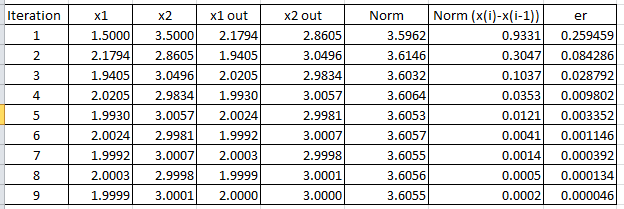
The following Microsoft Excel table shows that convergence to $x_1=2.0$ and $x_2=3.0$ satisfying the required criterion $\varepsilon_r<\varepsilon_s=0.0001$ is achieved after 9 iterations.

FPM

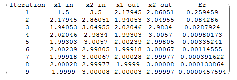
The following code does the same thing in Mathematica to produce the table below:

View Mathematica Code

xtable = {{1.5, 3.5}};
ErrorTable = {1};
Nmax = 100;
eps = 0.0001;
i = 2;
While[And[ErrorTable[[i - 1]] > eps, i <= Nmax], 
  x1new = Sqrt[10 - xtable[[i - 1, 1]]*xtable[[i - 1, 2]]]; 
  x2new = Sqrt[(57 - xtable[[i - 1, 2]])/3/x1new]; 
  xnew = {x1new, x2new};
  xtable = Append[xtable, xnew]; 
  er = Norm[xnew - xtable[[i - 1]]]/Norm[xnew]; 
  ErrorTable = Append[ErrorTable, er]; i = i + 1];
Title = {"Iteration", "x1_in", "x2_in", "x1_out", "x2_out", "Er"};
T2 = Table[{i, xtable[[i, 1]], xtable[[i, 2]], xtable[[i + 1, 1]], xtable[[i + 1, 2]], ErrorTable[[i + 1]]}, {i, 1, Length[xtable] - 1}];
T2 = Prepend[T2, Title];
T2 // MatrixForm

The example here shows that the fixed-point iteration method is not guaranteed to give a possible solution. In fact, the initial guess and the form chosen affect whether a solution can be obtained or not. Note that the “FixedPointList” built-in function in Mathematica can be used to implement the method with an initial guess. Notice in the code below how the function $g$ outputs the vector $x$ as a list and that the second component uses the output of the first component:

View Mathematica Code

g[x_] := (x1 = Sqrt[10 - x[[1]]*x[[2]]]; {x1, Sqrt[(57 - x[[2]])/3/x1]})
FixedPointList[g[#] &, {1.5, 3.5}, 20]

Newton-Raphson Method

The Newton-Raphson method is the method of choice for solving nonlinear systems of equations. Many engineering software packages (especially finite element analysis software) that solve nonlinear systems of equations use the Newton-Raphson method. The derivation of the method for nonlinear systems is very similar to the one-dimensional version in the root finding section. Assume a nonlinear system of equations of the form:

$\begin{split} f_1(x_1,x_2,\cdots,x_n)&=0\\ f_2(x_1,x_2,\cdots,x_n)&=0\\ &\vdots\\ f_n(x_1,x_2,\cdots,x_n)&=0 \end{split}$

If the components of one iteration $x^{(i)}\in\mathbb{R}^n$ are known as: $x_1^{(i)}, x_2^{(i)},\cdots,x_n^{(i)}$ , then, the Taylor expansion of the first equation around these components is given by:

$\begin{split} f_1\left(x_1^{(i+1)},x_2^{(i+1)},\cdots,x_n^{(i+1)}\right)\approx&f_1\left(x_1^{(i)},x_2^{(i)},\cdots,x_n^{(i)}\right)+\\ &\frac{\partial f_1}{\partial x_1}\bigg|_{x^{(i)}}\left(x_1^{(i+1)}-x_1^{(i)}\right)+\frac{\partial f_1}{\partial x_2}\bigg|_{x^{(i)}}\left(x_2^{(i+1)}-x_2^{(i)}\right)+\cdots+\\ &\frac{\partial f_1}{\partial x_n}\bigg|_{x^{(i)}}\left(x_n^{(i+1)}-x_n^{(i)}\right) \end{split}$

Applying the Taylor expansion in the same manner for $f_2, \cdots,f_n$ , we obtained the following system of linear equations with the unknowns being the components of the vector $x^{(i+1)}$ :

$\left(\begin{array}{c}f_1\left(x^{(i+1)}\right)\\f_2\left(x^{(i+1)}\right)\\\vdots \\ f_n\left(x^{(i+1)}\right)\end{array}\right) = \left(\begin{array}{c}f_1\left(x^{(i)}\right)\\f_2\left(x^{(i)}\right)\\\vdots \\ f_n\left(x^{(i)}\right)\end{array}\right)+ \left(\begin{matrix}\frac{\partial f_1}{\partial x_1}\big|_{x^{(i)}} & \frac{\partial f_1}{\partial x_2}\big|_{x^{(i)}} &\cdots&\frac{\partial f_1}{\partial x_n}\big|_{x^{(i)}} \\\frac{\partial f_2}{\partial x_1}\big|_{x^{(i)}} & \frac{\partial f_2}{\partial x_2}\big|_{x^{(i)}} & \cdots & \frac{\partial f_2}{\partial x_n}\big|_{x^{(i)}}\\\vdots&\vdots&\vdots&\vdots\\ \frac{\partial f_n}{\partial x_1}\big|_{x^{(i)}} & \frac{\partial f_n}{\partial x_2}\big|_{x^{(i)}} &\cdots& \frac{\partial f_n}{\partial x_n}\big|_{x^{(i)}} \end{matrix}\right)\left(\begin{array}{c}\left(x_1^{(i+1)}-x_1^{(i)}\right)\\\left(x_2^{(i+1)}-x_2^{(i)}\right)\\\vdots\\\left(x_n^{(i+1)}-x_n^{(i)}\right)\end{array}\right)$

By setting the left hand side to zero (which is the desired value for the functions $f_1, f_2, \cdots, f_n$ , then, the system can be written as:

$\left(\begin{matrix}\frac{\partial f_1}{\partial x_1}\big|_{x^{(i)}} & \frac{\partial f_1}{\partial x_2}\big|_{x^{(i)}} &\cdots&\frac{\partial f_1}{\partial x_n}\big|_{x^{(i)}} \\\frac{\partial f_2}{\partial x_1}\big|_{x^{(i)}} & \frac{\partial f_2}{\partial x_2}\big|_{x^{(i)}} & \cdots & \frac{\partial f_2}{\partial x_n}\big|_{x^{(i)}}\\\vdots&\vdots&\vdots&\vdots\\ \frac{\partial f_n}{\partial x_1}\big|_{x^{(i)}} & \frac{\partial f_n}{\partial x_2}\big|_{x^{(i)}} &\cdots& \frac{\partial f_n}{\partial x_n}\big|_{x^{(i)}} \end{matrix}\right)\left(\begin{array}{c}\left(x_1^{(i+1)}-x_1^{(i)}\right)\\\left(x_2^{(i+1)}-x_2^{(i)}\right)\\\vdots\\\left(x_n^{(i+1)}-x_n^{(i)}\right)\end{array}\right)= -\left(\begin{array}{c}f_1\left(x^{(i)}\right)\\f_2\left(x^{(i)}\right)\\\vdots \\ f_n\left(x^{(i)}\right)\end{array}\right)$

Setting $K_{ab}=\frac{\partial f_a}{\partial x_b}\big|_{x^{(i)}}$ , the above equation can be written in matrix form as follows:

$K \Delta x=-f$

where $K$ is an $n\times n$ matrix, $-f$ is a vector of $n$ components and $\Delta x$ is an $n$ -dimensional vector with the components $\left(x_1^{(i+1)}-x_1^{(i)}\right), \left(x_2^{(i+1)}-x_2^{(i)}\right),\cdots,\left(x_n^{(i+1)}-x_n^{(i)}\right)$ . If $K$ is invertible, then, the above system can be solved as follows:

$\Delta x = -K^{-1}f \Rightarrow x^{(i+1)}=x^{(i)}+\Delta x$

Example

Use the Newton-Raphson method with $\varepsilon_s=0.0001$ to find the solution to the following nonlinear system of equations:

$x_1^2+x_1x_2=10\qquad x_2+3x_1x_2^2=57$

Solution

In addition to requiring an initial guess, the Newton-Raphson method requires evaluating the derivatives of the functions $f_1=x_1^2+x_1x_2-10$ and $f_2=x_2+3x_1x_2^2-57$ . If $K_{ab}=\frac{\partial f_a}{\partial x_b}$ , then it has the following form:

$K=\left(\begin{matrix}\frac{\partial f_1}{\partial x_1}& \frac{\partial f_1}{\partial x_2}\\\frac{\partial f_2}{\partial x_1} & \frac{\partial f_2}{\partial x_2}\end{matrix}\right)=\left(\begin{matrix}2x_1+x_2& x_1\\3x_2^2 & 1+6x_1x_2\end{matrix}\right)$

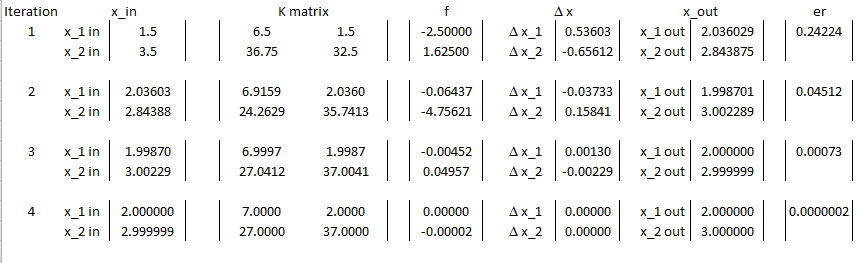
Assuming an initial guess of $x_1^{(0)}=1.5$ and $x_2^{(0)}=3.5$ , then the vector $f$ and the matrix $K$ have components:

$f=\left(\begin{array}{c}x_1^2+x_1x_2-10\\x_2+3x_1x_2^2-57\end{array}\right)=\left(\begin{array}{c}-2.5\\1.625\end{array}\right) \qquad K=\left(\begin{matrix}6.5 & 1.5 \\ 36.75 & 32.5\end{matrix}\right)$

The components of the vector $\Delta x$ can be computed as follows:

$\Delta x = -K^{-1}f=\left(\begin{array}{c}0.53603\\-0.65612\end{array}\right)$

Therefore, the new estimates for $x_1^{(1)}$ and $x_2^{(1)}$ are:

$x^{(1)}=x^{(0)}+\Delta x=\left(\begin{array}{c}2.036029\\2.843875\end{array}\right)$

The approximate relative error is given by:

$\varepsilon_r=\frac{\sqrt{(0.53603)^2+(-0.65612)^2}}{\sqrt{(2.036029)^2+(2.843875)^2}}=0.2422$

For the second iteration the vector $f$ and the matrix $K$ have components:

$f=\left(\begin{array}{c}-0.06437\\-4.75621\end{array}\right) \qquad K=\left(\begin{matrix}6.9159 & 2.0360 \\ 24.2629 & 35.7413\end{matrix}\right)$

The components of the vector $\Delta x$ can be computed as follows:

$\Delta x = -K^{-1}f=\left(\begin{array}{c}-0.03733\\0.15841\end{array}\right)$

Therefore, the new estimates for $x_1^{(2)}$ and $x_2^{(2)}$ are:

$x^{(2)}=x^{(1)}+\Delta x=\left(\begin{array}{c}1.998701\\3.002289\end{array}\right)$

The approximate relative error is given by:

$\varepsilon_r=\frac{\sqrt{(-0.03733)^2+(0.15841)^2}}{\sqrt{(1.998701)^2+(3.002289)^2}}=0.04512$

For the third iteration the vector $f$ and the matrix $K$ have components:

$f=\left(\begin{array}{c}-0.00452\\0.04957\end{array}\right) \qquad K=\left(\begin{matrix}6.9997 & 1.9987 \\ 27.0412 & 37.0041\end{matrix}\right)$

The components of the vector $\Delta x$ can be computed as follows:

$\Delta x = -K^{-1}f=\left(\begin{array}{c}0.00130\\-0.00229\end{array}\right)$

Therefore, the new estimates for $x_1^{(3)}$ and $x_2^{(3)}$ are:

$x^{(3)}=x^{(2)}+\Delta x=\left(\begin{array}{c}2.00000\\2.999999\end{array}\right)$

The approximate relative error is given by:

$\varepsilon_r=\frac{\sqrt{(0.00130)^2+(-0.00229)^2}}{\sqrt{(2.00000)^2+(2.999999)^2}}=0.00073$

Finally, for the fourth iteration the vector $f$ and the matrix $K$ have components:

$f=\left(\begin{array}{c}0.00000\\-0.00002\end{array}\right) \qquad K=\left(\begin{matrix}7 & 2 \\ 27 & 37\end{matrix}\right)$

The components of the vector $\Delta x$ can be computed as follows:

$\Delta x = -K^{-1}f=\left(\begin{array}{c}0.00000\\0.00000\end{array}\right)$

Therefore, the new estimates for $x_1^{(4)}$ and $x_2^{(4)}$ are:

$x^{(4)}=x^{(3)}+\Delta x=\left(\begin{array}{c}2\\3\end{array}\right)$

The approximate relative error is given by:

$\varepsilon_r=\frac{\sqrt{(0.00000)^2+(0.00000)^2}}{\sqrt{(2)^2+(3)^2}}=0.00000$

Therefore, convergence is achieved after 4 iterations which is much faster than the 9 iterations in the fixed-point iteration method. The following is the Microsoft Excel table showing the values generated in every iteration:

NR31

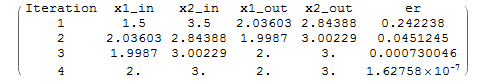
The Newton-Raphson method can be implemented directly in Mathematica using the “FindRoot” built-in function:
View Mathematica Code

FindRoot[{x1^2 + x1*x2 - 10 == 0, x2 + 3*x1*x2^2 == 57}, {{x1, 1.5}, {x2, 3.5}}]

The following “While” loop in Mathematica provides an iterative procedure that implements the Newton-Raphson Method in Mathematica and produces the table shown:
View Mathematica Code

x = {x1, x2};
f1 = x1^2 + x1*x2 - 10;
f2 = x2 + 3 x1*x2^2 - 57;
f = {f1, f2};
K = Table[D[f[[i]], x[[j]]], {i, 1, 2}, {j, 1, 2}];
K // MatrixForm
xtable = {{1.5, 3.5}};
xrule = {{x1 -> xtable[[1, 1]], x2 -> xtable[[1, 2]]}};
Ertable = {1}
NMax = 100;
i = 1;
eps = 0.000001

While[And[Ertable[[i]] > eps, i <= NMax], 
 Delta = -(Inverse[K].f) /. xrule[[i]]; 
 xtable = Append[xtable, Delta + xtable[[Length[xtable]]]]; 
 xrule = Append[
   xrule, {x1 -> xtable[[Length[xtable], 1]], 
    x2 -> xtable[[Length[xtable], 2]]}]; 
 er = Norm[Delta]/Norm[xtable[[i+1]]]; Ertable = Append[Ertable, er]; i++]
Title = {"Iteration", "x1_in", "x2_in", "x1_out", "x2_out", "er"};
T2 = Table[{i, xtable[[i, 1]], xtable[[i, 2]], xtable[[i + 1, 1]], xtable[[i + 1, 2]], Ertable[[i + 1]]}, {i, 1, Length[xtable] - 1}];
T2 = Prepend[T2, Title];
T2 // MatrixForm

Linear vs. Nonlinear Analysis of Structures: An Application

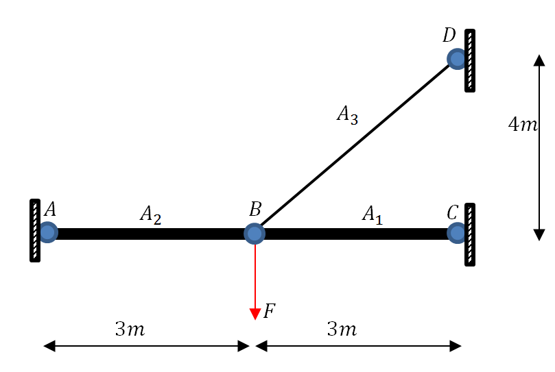
Most structural engineering problems in which the displacements and forces inside a structure are sought can be formulated using linear systems of equations. This is done by invoking certain assumptions that simplify the problem. However, when a structure undergoes large deformations, the problem has to be formulated using nonlinear systems of equations. The following is an example of a truss structure that aims at clarifying the difference.

Example

Two steel truss members with areas $A_1$ and $A_2$ are connected to a steel cable with an area $A_3$ as shown in the figure. All the connections are hinged connections allowing free relative rotations. Points $A$ , $C$ , and $D$ are fixed by means of hinges preventing displacements but allowing free rotations. Assuming that the horizontal displacement of point $B$ is $u_1$ to the right and the vertical displacement of point $B$ is $u_2$ downwards. Assume that Young’s modulus $E=200 GPa$ , $A_1=A_2=200 mm^2$ , and $A_3=50 mm^2$ . The force in each member is equal to $F_i=A_i\sigma_i=A_iE_i\varepsilon_i$ where $\varepsilon_i=\frac{L_i-L_{0i}}{L_{0i}}$ where $i=1,2,3$ is the member number, $L_{0i}$ is the undeformed length, $L_i$ is the deformed length, $\sigma_i$ is the longitudinal stress, $\varepsilon_i$ is the strain, and $E_i$ is Young’s modulus in member $i$ . Find the values of $u_1$ and $u_2$ at equilibrium using: 1) Linear analysis where the displacements are assumed to be small, and 2) Nonlinear analysis. Solve twice, once with $F=10,000 N$ , and another time with $F=500,000 N$ . Do the two solution strategies give the same answer?

structures1

Solution

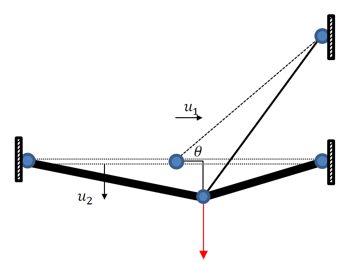
The units adopted will be $N$ for forces, $m$ for lengths, and $N/m^2$ for $E$ . The following is the displaced shape of the structure. The middle hinge move horizontally to the right a distance $u_1$ and vertically downards a distance $u_2$ . There are two unknowns in the problem $u_1$ and $u_2$ . These can be found using two equations of equilibrium at the middle hinge. The two equations are the sum of the vertical and horizontal forces, each equal to zero.
Structures2

Linear Analysis

In linear analysis, the truss member length is assumed to only change due to displacements along its longitudinal axis. In other words, the forces in the truss member do not change if it simply rotates. In addition, the forces are assumed to be aligned with the original geometry of the structure before deformations. The strains in each member are given by: $\varepsilon_1=\frac{3-u_1-3}{3}=\frac{-u_1}{3}$ , $\varepsilon_2=\frac{3+u_1-3}{3}=\frac{u_1}{3}$ , and $\varepsilon_3=\frac{5+u_2\sin{(\theta)}-u_1\cos{(\theta)}-5}{5}=\frac{u_2\sin{(\theta)}-u_1\cos{(\theta)}}{5}$ . Therefore, the forces in each member can be calculated as follows:

$\begin{split} F_1&=E_1A_1\varepsilon_1=E\left(\frac{200}{1000000}\right)\frac{-u_1}{3}\\ F_2&=E_2A_2\varepsilon_2=E\left(\frac{200}{1000000}\right)\frac{u_1}{3}\\ F_3&=E_3A_3\varepsilon_3=E\left(\frac{50}{1000000}\right)\frac{u_2\sin{(\theta)}-u_1\cos{(\theta)}}{5} \end{split}$

where $E=200(10^9) N/m^2$ , $\sin{\theta}=\frac{4}{5}$ , and $\cos{\theta}=\frac{3}{5}$ . Assuming small deformations, equilibrium at point $B$ can be analyzed using the following forces diagram:
Structures4
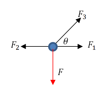
The first equation is the sum of horizontal forces equals to zero:

$F_1+F_3\cos{(\theta)}-F_2=\frac{-81260000}{3}u_1+960000u_2=0$

The second equation is the sum of the vertical forces equal to zero:

$F-F_3\sin{(\theta)}=F+960000u_1-1280000 u_2=0$

These equations are linear and can be written in matrix form as follows:

$\left(\begin{matrix} \frac{-81260000}{3} & 960000\\ 960000 & -1280000\end{matrix}\right)\left(\begin{array}{c} u_1\\u_2\end{array}\right)=\left(\begin{array}{c} 0\\-F\end{array}\right)$

Setting $F=10,000 N$ yields a solution $u_1=0.28mm$ and $u_2=8.02mm$ , while setting $F=500,000$ yields $u_1=14mm$ and $u_2=401mm$ . Notice that in a linear analysis, the displacements are directly proportional to the applied load, that is, the ratio between $u_1$ at $F=10,000$ and $u_1$ at $F=500,000$ is equal to $\frac{500,000}{10,000}$ . The same applies to $u_2$ .

The following is the Mathematica code to formulate and solve the above system of equations using the “Solve” function.
View Mathematica Code

Clear[F, Ee];
Ee = 200 (10^9);
eps1 = -u1/3;
A1 = A2 = 200/1000000;
A3 = 50/1000000;
eps2 = u1/3;
Cth = 3/5;
Sth = 4/5;
eps3 = (-u1*Cth + u2*Sth)/5;
F1 = Ee*A1*eps1;
F2 = Ee*A2*eps2;
F3 = Ee*A3*eps3;
Eq1 = Expand[(F1 + F3*Cth - F2)]
Eq2 = Expand[F - F3*Sth]
sol1 = Solve[{Eq1 == 0.0, Eq2 == 0.0 /. F -> 10000}]
sol2 = Solve[{Eq1 == 0.0, Eq2 == 0.0 /. F -> 500000}]

Nonlinear Analysis

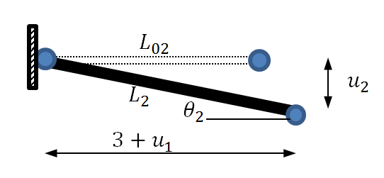
In a nonlinear analysis, the analysis takes into consideration the displaced position of the structure without any simplified assumptions. Looking at the first truss member, the displaced structure is shown in the following figure.
Structures5
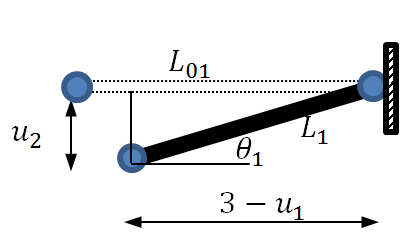
For this member, the original length $L_{01}=3$ , the final length $L_1=\sqrt{u_2^2+(3-u_1)^2}$ , the strain $\varepsilon_1=\frac{L_1-L_{01}}{L_{01}}$ and the angle of inclination $\theta_1$ is such that $\sin{(\theta_1)}=\frac{u_2}{L_1}$ and $\cos{(\theta_1)}=\frac{3-u_1}{L_1}$ .

For the second truss member, the displaced structure is shown in the following figure.
Structures6
For this member, the original length $L_{02}=3$ , the final length $L_2=\sqrt{u_2^2+(3+u_1)^2}$ , the strain $\varepsilon_2=\frac{L_2-L_{02}}{L_{02}}$ and the angle of inclination $\theta_2$ is such that $\sin{(\theta_2)}=\frac{u_2}{L_2}$ and $\cos{(\theta_2)}=\frac{3+u_1}{L_2}$ .

For the third truss member, the displaced structure is shown in the following figure.
structures9
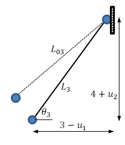
For this member, the original length $L_{03}=5$ , the final length $L_3=\sqrt{(4+u_2)^2+(3-u_1)^2}$ , the strain $\varepsilon_3=\frac{L_3-L_{03}}{L_{03}}$ and the angle of inclination $\theta_3$ is such that $\sin{(\theta_3)}=\frac{4+u_2}{L_3}$ and $\cos{(\theta_3)}=\frac{3-u_1}{L_3}$ .

Finally, the equations of equilibrium can be written taking into consideration the inclination of each member:
Structures8
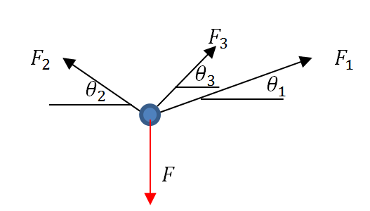
The first equation is the sum of horizontal forces equals to zero:

$F_1\cos{(\theta_1)}+F_3\cos{(\theta_3)}-F_2\cos{(\theta_2)}=0$

The second equation is the sum of the vertical forces equal to zero:

$F-F_1\sin{(\theta_1)}-F_2\sin{(\theta_2)}-F_3\sin{(\theta_3)}=0$

The following is a screenshot of the Mathematica output of the two equations:
Structures10

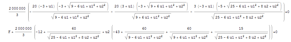
Setting $F=10,000 N$ yields a solution $u_1=0.28mm$ and $u_2=8.02mm$ , while setting $F=500,000 N$ yields $u_1=11.6mm$ and $u_2=340mm$ . For small deformations under small applied loads, the linear analysis and nonlinear analysis produce exactly the same results. In this situation, the rotations of the members are very small such that the original shape and the deformed shape can be assumed to be the same. However, under large loads, the linear analysis is no longer valid. The two solutions at $F=500,000 N$ are far from each other with the nonlinear analysis solution giving less displacement. In this particular situation, as the structure deforms, the nonlinear effects cause the structure to be more rigid and therefore exhibit less deformations. Cable structures with large loads and large deformations in the cables need to be analyzed using a nonlinear analysis rather than a linear analysis.

The following is the Mathematica code to formulate and solve the above nonlinear system of equations using the “FindRoot” function with an initial guess of $u_1=0$ , and $u_2=0$ .

View Mathematica Code

Ee = 200 (10^9);
A1 = A2 = 200/1000000;
A3 = 50/1000000;
L1 = Sqrt[(3 - u1)^2 + u2^2];
Sth1 = u2/L1;
Cth1 = (3 - u1)/L1;
L2 = Sqrt[(3 + u1)^2 + u2^2];
Sth2 = u2/L2;
Cth2 = (3 + u1)/L2;
L3 = Sqrt[(3 - u1)^2 + (4 + u2)^2];
Cth3 = (3 - u1)/L3;
Sth3 = (4 + u2)/L3;
eps1 = (L1 - 3)/3;
eps2 = (L2 - 3)/3;
eps3 = (L3 - 5)/5;
F1 = Ee*A1*eps1;
F2 = Ee*A2*eps2;
F3 = Ee*A3*eps3;
Eq1 = Simplify[F1*Cth1 - F2*Cth2 + F3*Cth3]
Eq2 = Simplify[F - F1*Sth1 - F2*Sth2 - F3*Sth3]

sol1 = FindRoot[{Eq1 == 0, Eq2 == 0 /. F -> 10000}, {{u1, 0}, {u2, 0}}]
sol2 = FindRoot[{Eq1 == 0, Eq2 == 0 /. F -> 500000}, {{u1, 0}, {u2, 0}}]

Problems

Use your implementation of the Newton-Raphson method to find 4 different sets of roots for the following nonlinear system of equations:
$\begin{split} 4-2x_1^2-x_2&=0\\ 8-4x_1-x_2^2&=0 \end{split}$

Use $\varepsilon_s=0.0001$ . Compare with the “FindRoot” built-in function in Mathematica.
Use your implementation of the Newton-Raphson method to find 1 set of roots for the following nonlinear system of equations:
$\begin{split} y=-x^2+x+0.5\\ y+5xy=x^2 \end{split}$

Use $\varepsilon_s=0.0001$ . Compare with the “FindRoot” built-in function in Mathematica.
Compare the convergence of the Newton-Raphson method and the fixed-point iteration method with initial guesses of $x=y=1.5$ and $\varepsilon_s=0.0001$ to find a solution to the following nonlinear system of equations:

$\begin{split} x^2=5-y^2\\ y+1=x^2 \end{split}$
Use the Newton-Raphson method to find a solution to the following nonlinear set of equations:

$\begin{split} 20x_1^4x_2+3x_2^3=20\\ 20x_1^2x_2^3=1 \end{split}$

Use $\varepsilon_s=0.0001$
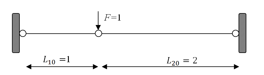
The following structural system is composed of two truss elements with unit cross sectional area. The left and right supports are hinged supports. The middle connection where the load is applied is also a hinged connection. Find the displacement at equilibrium of the following structural system. Assume a linear material with $\sigma=10\varepsilon$ where $\sigma$ is the stress in the bar, $\varepsilon=\frac{\Delta L}{L_0}$ is the corresponding strain, and $L_0$ is the initial length. Use the Newton-Raphson method.
Solve the following nonlinear system of equations using the Newton-Raphson method and $\varepsilon_s=0.0001$
$\begin{split} x_1-x_2-x_3-0.2=0\\ x_2-x_4-0.2=0\\ x_4+x_5-0.2=0\\ -x_5-x_6+x_7-0.2=0\\ x_3+x_6-0.2=0\\ 20|x_2|x_2-30|x_3|x_3+20|x_4|x_4-20|x_5|x_5+40|x_6|x_6=0\\ 60|x_1|x_1+30|x_3|x_3-40|x_6|x_6-30|x_7|x_7-10=0 \end{split}$

Hint, if $x_i\neq 0$ :

$\frac{\partial |x_i|x_i}{\partial x_i}=2|x_i|$