Engineering at Alberta Courses » Linear Systems of Equations

Introduction to Numerical Analysis: Linear Systems of Equations

Definitions

Linear Vector Spaces

In this course, by a linear vector space we mean the set

$\mathbb{R}^n=\mathbb{R}\times\mathbb{R}\times\cdots\mathbb{R}=\left\{\left(\begin{array}{c}x_1\\x_2\\\vdots\\x_n\end{array}\right)\bigg| x_1,x_2,\cdots,x_n\in\mathbb{R} \right\}$

The dimension of this vector space is $n$ . A vector in this space $x\in\mathbb{R}^n$ has $n$ components $x_1, x_2,\cdots,x_n$ each of which is a real number. The zero vector is the vector whose components are all equal to zero.

For example $\mathbb{R}^2$ is the two-dimensional linear vector space. Each vector in this space has two components. $\mathbb{R}^2$ can be represented geometrically by a plane. $\mathbb{R}^3$ is a three-dimensional linear vector space. Each vector in this space has three components. The vector $\left(\begin{array}{c}0\\0\end{array}\right)$ is the zero vector in $\mathbb{R}^2$ . The vector $\left(\begin{array}{c}0\\0\\0\end{array}\right)$ is the zero vector in $\mathbb{R}^3$ .

Linear Functions between Vector Spaces(Matrices)

Given a linear vector space $\mathbb{R}^m$ , and another linear vector space $\mathbb{R}^n$ , a linear function $f:\mathbb{R}^m\rightarrow\mathbb{R}^n$ has the following form, $\forall x\in\mathbb{R}^m$ :

$f(x)=\left(\begin{array}{c} a_{11}x_1+a_{12}x_2+\cdots +a_{1m}x_m\\ a_{21}x_1+a_{22}x_2+\cdots +a_{2m}x_m\\ \vdots \\ a_{n1}x_1+a_{n2}x_2+\cdots +a_{nm}x_m \end{array}\right)$

The function $f$ takes a vector $x$ with $m$ components and returns a vector $y=f(x)$ which has $n$ components. Using matrix notation, the above can be written in the following more convenient form:

$f(x)=\left(\begin{matrix}a_{11}&a_{12}&\cdots&a_{1m}\\a_{21}&a_{22}&\cdots&a_{2m}\\\vdots&\vdots&\vdots&\vdots\\a_{n1}&a_{n2}&\cdots&a_{nm}\end{matrix}\right)\left(\begin{array}{c}x_1\\x_2\\\vdots\\x_m\end{array}\right)$

If we denote the $n\times m$ matrix of numbers by $A$ , then the linear function $f$ can be written in the following simple form:

$f(x)=Ax$

We noted that $x$ is an element of the linear vector space $\mathbb{R}^m$ . Similarly, we view $A$ as an element of the possible linear functions from $\mathbb{R}^m$ to $\mathbb{R}^n$ which is denoted: $\mathbb{B}(\mathbb{R}^m,\mathbb{R}^n)$

If $n=m$ , then for simplicity, we say that $A\in\mathbb{B}(\mathbb{R}^n)$ . We also use the symbol $\mathbb{M}^n$ to denote the set of square matrices that live in the space $\mathbb{B}(\mathbb{R}^n)$ .

For a visual representation showing the action of the matrix $A\in\mathbb{M}^2$ on the space $\mathbb{R}^2$ , see the tool shown here.

Matrix Transpose

If $A\in\mathbb{B}(\mathbb{R}^m,\mathbb{R}^n)$ , then the transpose of $A$ , namely $A^T$ is defined as the matrix $A^T\in\mathbb{B}(\mathbb{R}^n,\mathbb{R}^m)$ whose columns are the rows of $A$ .

Examples

Example 1

Consider the function $f:\mathbb{R}\rightarrow\mathbb{R}$ defined as $f(x)=5x$ . Following the above definition, $x$ is a one-dimensional vector and the matrix $A$ has dimensions $1\times 1$ . In this case $A\in \mathbb{B}(\mathbb{R}^1)$ and $A=A^T$ .

Example 2

Consider the function $f:\mathbb{R}^3\rightarrow\mathbb{R}^2$ defined as follows: $\forall x\in\mathbb{R}^3$ :

$f(x)=\left(\begin{array}{c}5x_1+3x_2+2x_3\\2x_2+4x_3\end{array}\right)$

In matrix form, this function can be represented as follows:

$f(x)=\left(\begin{array}{ccc}5&3&2\\0&2&4\end{array}\right)\left(\begin{array}{c}x_1\\x_2\\x_3\end{array}\right)$

This function takes vectors that have three components and gives vectors that have two components. The matrix $A$ associated with this linear function has dimensions $2\times 3$ , lives in the space $\mathbb{B}(\mathbb{R}^3,\mathbb{R}^2)$ , and has the form:

$A=\left(\begin{array}{ccc}5&3&2\\0&2&4\end{array}\right)$

In this case, $A^T$ is simply:

$A^T=\left(\begin{array}{cc}5&0\\3&2\\2&4\end{array}\right)$

Example 3

Consider the function $f:\mathbb{R}^3\rightarrow\mathbb{R}^3$ defined as follows: $\forall x\in\mathbb{R}^3$ :

$f(x)=\left(\begin{array}{c}5x_1+3x_2+2x_3\\2x_2+4x_3\\2x_1-3x_3\end{array}\right)$

In matrix form, this function can be represented as follows:

$f(x)=\left(\begin{array}{ccc}5&3&2\\0&2&4\\2&0&-3\end{array}\right)\left(\begin{array}{c}x_1\\x_2\\x_3\end{array}\right)$

This function takes vectors that have three components and gives vectors that have three components. The matrix $A$ associated with this linear function has dimensions $3\times 3$ , lives in the space $\mathbb{B}(\mathbb{R}^3)=\mathbb{M}^3$ , and has the form:

$A=\left(\begin{array}{ccc}5&3&2\\0&2&4\\2&0&-3\end{array}\right)$

In this case, $A^T$ is simply:

$A^T=\left(\begin{array}{ccc}5&0&2\\3&2&0\\2&4&-3\end{array}\right)$

Example 4

Consider the function $f:\mathbb{R}^3\rightarrow\mathbb{R}$ defined as follows: $\forall x\in\mathbb{R}^3$ :

$f(x)=\left(\begin{array}{c}5x_1+2x_3\end{array}\right)$

In matrix form, this function can be represented as follows:

$f(x)=\left(\begin{array}{ccc}5&0&2\end{array}\right)\left(\begin{array}{c}x_1\\x_2\\x_3\end{array}\right)$

This function takes vectors that have three components and gives vectors that have one component. The matrix $A$ associated with this linear function has dimensions $1\times 3$ , lives in the space $\mathbb{B}(\mathbb{R}^3,\mathbb{R})$ , and has the form:

$A=\left(\begin{array}{ccc}5&0&2\end{array}\right)$

In this case, $A^T$ is simply:

$A^T=\left(\begin{array}{c}5\\0\\2\end{array}\right)$

Linear System of Equations

Let $A\in\mathbb{B}(\mathbb{R}^m,\mathbb{R}^n)$ and given a vector $b\in\mathbb{R}^n$ , a linear system of equations seeks the solution $x$ to the equation:

$Ax=b$

In a matrix component form the above equation is:

$\left(\begin{matrix}a_{11}&a_{12}&\cdots&a_{1m}\\a_{21}&a_{22}&\cdots&a_{2m}\\\vdots&\vdots&\vdots&\vdots\\a_{n1}&a_{n2}&\cdots&a_{nm}\end{matrix}\right)\left(\begin{array}{c}x_1\\x_2\\\vdots\\x_m\end{array}\right)=\left(\begin{array}{c}b_1\\b_2\\\vdots\\b_n\end{array}\right)$

Another way of viewing this set of equations is as follows:

$\begin{split} a_{11}x_1+a_{12}x_2+\cdots +a_{1m}x_m&=b_1\\ a_{21}x_1+a_{22}x_2+\cdots +a_{2m}x_m&=b_2\\ &\vdots \\ a_{n1}x_1+a_{n2}x_2+\cdots +a_{nm}x_m&=b_n \end{split}$

The solution for a linear system of equations is the numerical value for the variables $x_1, x_2,\cdots,x_m$ that would satisfy the above equations. There are three possible scenarios:

Scenario 1

If $m>n$ then we have more unknown components of the $m$ -dimensional vector $x$ than we have equations. The system is then termed underdetermined. This results in having many possible solutions. For example, consider the linear system of equations $Ax=b$ defined as:

$\left(\begin{array}{ccc}5&3&2\\0&2&4\end{array}\right)\left(\begin{array}{c}x_1\\x_2\\x_3\end{array}\right)=\left(\begin{array}{c}1\\2\end{array}\right)$

There are many possible solutions that would satisfy the above equation. One solution can be obtained by setting $x_3=1$ . Then:

$\begin{split} 5x_1+3x_2+2&=1\\ 2x_2+4&=2 \end{split}$

which results in $x_2=-1$ and $x_1=\frac{2}{5}$ . Therefore one possible solution is:

$x=\left(\begin{array}{c}\frac{2}{5}\\-1\\1\end{array}\right)$

Another possible solution can be obtained by setting $x_3=2$ . Then:

$\begin{split} 5x_1+3x_2+4&=1\\ 2x_2+8&=2 \end{split}$

which results in $x_2=-3$ and $x_1=\frac{6}{5}$ . Therefore another possible solution is:

$x=\left(\begin{array}{c}\frac{6}{5}\\-3\\2\end{array}\right)$

In fact, there are infinite possible solutions that depend on what value you choose for $x_3$ . So, if $x_3$ is set such that $x_3=\alpha$ , then we have:

$\begin{split} 5x_1+3x_2+2\alpha&=1\\ 2x_2+4\alpha&=2 \end{split}$

Therefore:

$x_2=\frac{2-4\alpha}{2}=1-2\alpha$

and

$x_1=\frac{1}{5}(1-2\alpha - 3(1-2\alpha))=\frac{1}{5}(-2+4\alpha)$

Therefore:

$x=\left(\begin{array}{c}\frac{-2+4\alpha}{5}\\1-2\alpha\\\alpha\end{array}\right)$

Scenario 2

If $m<n$ and the $n$ equations are linearly independent, then we have more equations than we have unknown components of the $m$ -dimensional vector $x$ . This results in having too many restrictions which prevents us from finding a solution. In this case, the system is termed overdetermined. For example, consider the linear system of equations $Ax=b$ defined as:

$\left(\begin{array}{cc}1&3\\0&2\\-1&1\end{array}\right)\left(\begin{array}{c}x_1\\x_2\end{array}\right)=\left(\begin{array}{c}1\\2\\2\end{array}\right)$

In this system, we have three independent equations and two unknowns $x_1$ and $x_2$ . If the first two equations are used to find a solution, then the third equation will present a contradiction. The first two equations have the following form:

$\begin{split} x_1+3x_2&=1\\ 2x_2&=2 \end{split}$

which result in the solution $x_2=1$ , and $x_1=-2$ . If we substitute this solution into equation 3 we get:

$-1\times (-2)+1\times 1=2+1=3\neq 2$

Scenario 3

If $m=n$ and the $n$ equations are independent, i.e., the rows of the matrix are linearly independent, then one unique solution exists and the matrix $A$ that forms the equation has an inverse. In this case, there exists a matrix $A^{-1}$ such that:

$Ax=b\Rightarrow x=A^{-1}b$

To know whether the equations are independent or not the determinant function defined below is sufficient. If the determinant of a matrix is equal to 0, then the rows of the matrix are linearly dependent, and so, an inverse cannot be found. If the determinant of a matrix on the other hand is not equal to 0, then the rows of the matrix are linearly independent and an inverse can be found.

For example, consider the system $Ax=b$ defined as:

$\left(\begin{array}{cc}1&3\\0&2\end{array}\right)\left(\begin{array}{c}x_1\\x_2\end{array}\right)=\left(\begin{array}{c}1\\2\end{array}\right)$

The rows of the matrix $A$ are clearly linearly independent. The inverse of $A$ can be found (which will be discussed later in more detail). For now, we can simply solve the two equations as follows. From the second equation we get:

$2x_2=2\Rightarrow x_2=1$

Substituting into the first equation we get:

$x_1+3(1)=1\Rightarrow x_1=-2$

Therefore, the system has a unique solution.

If $m=n$ and the $n$ equations are dependent, i.e., the rows of the matrix are linearly dependent, then it is not possible to find a unique solution for the linear system of equations. For example, consider the system $Ax=b$ defined as:

$\left(\begin{array}{cc}1&1\\-1&-1\end{array}\right)\left(\begin{array}{c}x_1\\x_2\end{array}\right)=\left(\begin{array}{c}1\\2\end{array}\right)$

The rows of the matrix $A$ are clearly linearly dependent. The inverse of $A$ can not be found (which will be discussed later in more detail). The system presents a contradiction and cannot be solved because the first equation predicts that $x_1+x_2=1$ while the second equation predicts that $x_1+x_2=-2$ !

As a different example, consider the system $Ax=b$ defined as:

$\left(\begin{array}{cc}1&1\\-1&-1\end{array}\right)\left(\begin{array}{c}x_1\\x_2\end{array}\right)=\left(\begin{array}{c}1\\-1\end{array}\right)$

The rows of the matrix $A$ are clearly linearly dependent. The inverse of $A$ can not be found (which will be discussed later in more detail). The system has infinite number of possible solutions. The first and second equations give us the relationship $x_2=1-x_1$ . So, by assuming any value for $x_1$ , we can find a value for $x_2$ . For example, if $x_1=1$ , then $x_2=0$ . Another possible solution is $x_1=0$ and $x_2=1$ .

We will focus in the remaining part of this section on how to find a solution for a linear system of equations when $m=n$ .

Special Types of Square Matrices

Symmetric Matrix

A symmetric matrix $A$ is a matrix that satisfies $A=A^T$ . For example:

$A=\left(\begin{array}{cc}1&3\\3&2\end{array}\right)$

is a symmetric matrix.

Identity Matrix

The identity matrix $I\in\mathbb{M}^n$ is the matrix whose diagonal components have the value of 1 while its off diagonal components have a value of zero. For example, $I\in\mathbb{M}^3$ has the form:

$I=\left(\begin{array}{ccc}1&0&0\\0&1&0\\0&0&1\end{array}\right)$

This is called the identity matrix because it takes every vector $x$ and returns the same vector. For example, consider the general vector $x\in\mathbb{R}^3$ with components $x_1$ , $x_2$ , and $x_3$ . The same vector is obtained after the operation $Ix$ :

$Ix=\left(\begin{array}{ccc}1&0&0\\0&1&0\\0&0&1\end{array}\right)\left(\begin{array}{c}x_1\\x_2\\x_3\end{array}\right)=\left(\begin{array}{c}x_1\\x_2\\x_3\end{array}\right)=x$

Diagonal Matrix

A matrix $M\in\mathbb{M}^n$ is called diagonal if all its off diagonal components are zero. The identity matrix is a diagonal matrix. Similarly, the following matrix is diagonal:

$M=\left(\begin{array}{cccc}5&0&0&0\\0&-1&0&0\\0&0&0&0\\0&0&0&-3\end{array}\right)$

Upper Triangular Matrix

Let $M\in\mathbb{M}^n$ . $M$ is an upper triangular matrix if all the components below the diagonal components are equal to zero. For example, the following matrix is an upper triangular matrix:

$M=\left(\begin{matrix}1&2&3\\0&1&4\\0&0&5\end{matrix}\right)$

Lower Triangular Matrix

Let $M\in\mathbb{M}^n$ . $M$ is a lower triangular matrix if all the components above the diagonal components are equal to zero. For example, the following matrix is a lower triangular matrix:

$M=\left(\begin{matrix}1&0&0&0\\5&2&0&0\\2&3&1&0\\1&2&0&3\end{matrix}\right)$

Banded Matrix

A matrix $M\in\mathbb{M}^n$ is called banded if all its components are zero except the components on the main diagonal and one or more diagonals on either side. The band width is the maximum number of columns on the same row that have non-zero entries. For example, the following $M\in\mathbb{M}^5$ is banded with a band width of 3.

$M=\left(\begin{matrix}1&0&0&0&0\\1&2&3&0&0\\0&3&1&2&0\\0&0&1&2&3\\0&0&0&4&4\end{matrix}\right)$

Matrix Operations

Matrix Addition

Let $M_1,M_2\in\mathbb{M}^n$ . Consider the function $f_1(x)=M_1x$ and the function $f_2(x)=M_2x$ . Then, the function $f_3(x)=f_1(x)+f_2(x)$ is given as:

$f_3(x)=M_1x+M_2x=(M_1+M_2)x=M_3x$

where $M_3=M_1+M_2$ is computed by adding each component in $M_1$ to the corresponding component in $M_2$ . For example, consider the two matrices:

$M_1=\left(\begin{matrix}5&2\\0&1\end{matrix}\right) \qquad M_2=\left(\begin{matrix}-1&0\\2&2\end{matrix}\right)$

Then, the matrix $M_3$ can be computed as follows:

$M_3=M_1+M_2=\left(\begin{matrix}4&2\\2&3\end{matrix}\right)$

Two matrices can only be added if they have the same dimensions.

Matrix Multiplication

Consider the matrix $M\in\mathbb{B}(\mathbb{R}^m,\mathbb{R}^n)$ which takes vectors of dimensions $m$ and returns vectors of dimensions $n$ . The matrix $M$ has dimensions $n\times m$ . Consider the matrix $N\in\mathbb{B}(\mathbb{R}^n,\mathbb{R}^l)$ which takes vectors of dimension $n$ and gives vectors of dimension $l$ . The matrix $N$ has dimensions $l\times n$ . The combined operation $N(M(x))$ takes vectors of dimensions $m$ and gives vectors of dimension $l$ . This matrix $L=NM$ corresponding to the combined operation can be obtained by taking the dot product of the row vectors of the matrix $N$ with the column vectors of the matrix $M$ . This can only be done if the inner dimensions are equal to each other. The product $L=NM$ would have dimensions of $l\times m$ and it is such that $L\in\mathbb{B}(\mathbb{R}^m,\mathbb{R}^l)$ :

$L_{l\times m}=N_{l\times n}M_{n\times m}$

For example, consider the two matrices:

$N=\left(\begin{array}{cc}1&4\\2&2\\3&5\end{array}\right) \qquad M=\left(\begin{array}{cccc}2&3&1&5\\0&-1&2&4\end{array}\right)$

We can only perform the operation $L=NM$ but the opposite is not defined. The matrix multiplication $L=NM$ results in:

$L=\left(\begin{array}{cccc} 1\times 2+ 4\times 0 & 1\times 3-4\times 1 & 1\times 1+4\times 2 & 1\times 5 + 4\times 4\\ 2\times 2+ 2\times 0 & 2\times 3-2\times 1 & 2\times 1+2\times 2 & 2\times 5 + 2\times 4\\ 3\times 2+ 5\times 0 & 3\times 3-5\times 1 & 3\times 1+5\times 2 & 3\times 5 + 5\times 4 \end{array}\right)=\left(\begin{array}{cccc}2&-1&9&21\\4&4&6&18\\6&4&13&35\end{array}\right)$

You can use “.” in Mathematica to multiply matrices, or you can use “MMULT” in excel to multiply matrices.
View Mathematica Code

Nn = {{1, 4}, {2, 2}, {3, 5}};
M = {{2, 3, 1, 5}, {0, -1, 2, 4}};
L = Nn.M;
L // MatrixForm

It is important to note that when the dimensions are appropriate, then matrix multiplication is associative and distributive, i.e., given the three matrices $A,B,C$ then:

$A(BC)=(AB)C \qquad A(B+C)=AB+AC$

However, matrix multiplication is not necessarily commutative, i.e., $AB\neq BA$ . For example, consider the matrices

$A=\left(\begin{array}{cc}1&2\\0&0\end{array}\right) \qquad B=\left(\begin{array}{cc}1&1\\-1&1\end{array}\right)$

Then:

$AB=\left(\begin{array}{cc}-1&3\\0&0\end{array}\right) \neq BA=\left(\begin{array}{cc}1&2\\-1&-2\end{array}\right)$

Matrix Determinant

If $M\in\mathbb{M}^2$ such that:

$M=\left(\begin{matrix}a_1 &a_2\\b_1 & b_2\end{matrix}\right)$

then $\det{M}=a_1b_2-a_2b_1$ . If $M\in\mathbb{M}^3$ such that:

$M=\left(\begin{matrix}a_1 &a_2&a_3\\b_1 & b_2&b_3\\c_1&c_2&c_3\end{matrix}\right)$

then $\det{M}=a_1(b_2c_3-b_3c_2)+a_2(b_3c_1-b_1c_3)+a_3(b_1c_2-b_2c_1)$ .

Let $M\in\mathbb{M}^n$ . The matrix determinant can be defined using the recursive relationship:

$\det{M}=\sum_{i=1}^n(-1)^{(i+1)}M_{1i}\det{N_i}$

where $N_i\in\mathbb{M}^{n-1}$ and is formed by eliminating the 1st row and $i^{th}$ column of the matrix $M$ . It can be shown that $\det{M}=0\Leftrightarrow$ the rows of $M$ are linearly dependent. In other words, $\det{M}=0$ if and only if the matrix cannot be inverted. The function “Det[]” in Mathematica can be used to calculate the determinant of a matrix. In Excel, you can use the function “MDETERM()” to calculate the determinant of a matrix as well.

The following function in Mathematica computes the determinant of the matrix using the above recursive relationship and then compares the solution with the built-in function “Det[]” in Mathematica.
View Mathematica Code

fdet[M_] := (n = Length[M]; If[n == 2, (M[[1, 1]]*M[[2, 2]] - M[[1, 2]]*M[[2, 1]]),Sum[(-1)^(i + 1) M[[1, i]]*fdet[Drop[M, 1, {i}]], {i, 1, n}]]);
M = {{1, 1, 3, 7}, {4, 4, 5, 0}, {1, 5, 5, 6}, {1, -4, 3, -2}};
fdet[M]
Det[M]

You can check the section on the determinant of a matrix for additional information on some of the properties of the determinant of a matrix.

Solving Systems of Linear Equations

Solving systems of linear equations has been the subject of study for many centuries. In particular, for every engineering discipline and almost every engineering application, systems of linear equations appear naturally with large numbers of unknowns. For example, the stiffness method in structural analysis as well as the finite element analysis method seek to find the solution of the linear system of equations $Ku=f$ where $K$ is a symmetric matrix of dimensions $n\times n$ , $f\in\mathbb{R}^n$ is a vector of external forces and $u$ is the vector of the displacement of the structure nodes. The software used need to implement a method by which $u$ can be obtained given particular values for $f$ . An appropriate method to solve for a linear system of equations has to be computationally efficient. In the following, we will present a few methods to solve systems in which the number of equations is equal to the number of unknowns along with their pros and cons.

Cramer’s Rule

Cramer’s rule is one of the early methods to solve systems of linear equations $Ax=b$ . It is dated back to the eighteenth century! The method works really well; however, it is inefficient when the number of equations is very large. Nevertheless, with the current computing capabilities, the method can still be pretty fast. The method works using the following steps. First, the determinant of the matrix $A$ is calculated. Each component $x_i$ of the unknowns can be computed as:

$x_i=\frac{\det{D_i}}{\det{A}}$

where $D_i$ is the matrix formed by replacing the $i^{th}$ column in $A$ with the vector $b$ .

Example 1

Consider the linear system of equations $Ax=b$ defined as:

$\left(\begin{matrix}1&2\\-2&1\end{matrix}\right)\left(\begin{array}{c}x_1\\x_2\end{array}\right)=\left(\begin{array}{c}-1\\2\end{array}\right)$

$\det{A}=1\times 1 + 2\times 2=5$ . We will form the following two matrices by replacing the first column in $A$ with $b$ and then the second column in $A$ with $b$ :

$D_1=\left(\begin{matrix}-1&2\\2&1\end{matrix}\right) \qquad D_2=\left(\begin{matrix}1&-1\\-2&2\end{matrix}\right)$

The determinants of these matrices are:

$\det{D_1}=-1\times 1-2\times 2=-5 \qquad \det{D_2}=1\times 2-2\times 1=0$

Therefore:

$x_1=\frac{\det{D_1}}{\det{A}}=\frac{-5}{5}=-1 \qquad x_2=\frac{\det{D_2}}{\det{A}}=\frac{0}{5}=0$

The following is code that can be used for Cramer’s rule for a two-dimensional system of equations.

View Mathematica Code

A = {{a11, a12}, {a21, a22}};
AT = Transpose[A]
b = {b1, b2};
s1 = Drop[AT, {1}]
s2 = Drop[AT, {2}]
D1T = Insert[s1, b, 1]
D2T = Insert[s2, b, 2]
D1 = Transpose[D1T]
D2 = Transpose[D2T]
x1 = Det[D1]/Det[A]
x2 = Det[D2]/Det[A]

Example 2

Consider the linear system of equations $Ax=b$ defined as:

$\left(\begin{matrix}1&2&3\\2&1&4\\1&3&5\end{matrix}\right)\left(\begin{array}{c}x_1\\x_2\\x_3\end{array}\right)=\left(\begin{array}{c}-4\\8\\0\end{array}\right)$

$\det{A}=-4$ . We will form the following three matrices by replacing the corresponding columns in $A$ with $b$ :

$D_1=\left(\begin{matrix}-4&2&3\\8&1&4\\0&3&5\end{matrix}\right) \qquad D_2=\left(\begin{matrix}1&-4&3\\2&8&4\\1&0&5\end{matrix}\right) \qquad D_3=\left(\begin{matrix}1&2&-4\\2&1&8\\1&3&0\end{matrix}\right)$

The determinants of these matrices are:

$\det{D_1}=20 \qquad \det{D_2}=40 \qquad \det{D_3}=-28$

Therefore:

$x_1=\frac{\det{D_1}}{\det{A}}=-5 \qquad x_2=\frac{\det{D_2}}{\det{A}}=-10 \qquad x_3=\frac{\det{D_3}}{\det{A}}=7$

The following procedure applies the Cramer’s rule to a general system. Test the procedure to see how fast it is for higher dimensions.
View Mathematica Code

Cramer[A_, b_] := (n = Length[A];
  Di = Table[A, {i, 1, n}];
  Do[Di[[i]][[All, i]] = b, {i, 1, n}];
  x = Table[Det[Di[[i]]]/Det[A], {i, 1, n}])

A = {{1, 2, 3, 5}, {2, 0, 1, 4}, {1, 2, 2, 5}, {4, 3, 2, 2}};
b = {-4, 8, 0, 10};
Cramer[A, b]

The following link provides the MATLAB code for implementing the Cramer’s rule.

MATLAB file Download

Naive Gauss Elimination

The naive Gauss elimination is a procedure in which the linear system of equations is manipulated such that the coefficients of the component $x_i$ are eliminated from equation $i+1$ to equation $n$ . It would then be possible to solve for $x_n$ using the last equation, and then backward substitute to find the remaining components. The procedure is divided into two steps, forward elimination followed by backward substitution. We will illustrate the process in the following example. Consider the system of equations $Ax=b$ defined as:

$\begin{split} 2x_1+2x_2+2x_3&=6\\ 2x_1+3x_2+4x_3&=4\\ -x_1+2x_2+3x_3&=8\\ \end{split}$

Forward elimination: First, we will use the first equation to eliminate the coefficients of $x_1$ in equation 2 and 3. By multiplying the first equation by -1 and adding it to the second equation we get:

$\begin{split} 2x_1+2x_2+2x_3&=6\\ (2-2)x_1+(3-2)x_2+(4-2)x_3&=(4-6)\\ -x_1+2x_2+3x_3&=8\\ \end{split}$

which becomes:

$\begin{split} 2x_1+2x_2+2x_3&=6\\ 0+1x_2+2x_3&=-2\\ -x_1+2x_2+3x_3&=8\\ \end{split}$

By multiplying the first equation by $\frac{1}{2}$ and adding it to the third equation we get:

$\begin{split} 2x_1+2x_2+2x_3&=6\\ 0+1x_2+2x_3&=-2\\ 0+3x_2+4x_3&=11\\ \end{split}$

We are now ready to eliminate the coefficient of $x_2$ from equation 3 by multiplying equation 2 by -3 and adding it to equation 3:

$\begin{split} 2x_1+2x_2+2x_3&=6\\ 0+1x_2+2x_3&=-2\\ 0+0-2x_3&=17\\ \end{split}$

Backward substitution: Solving the above system becomes very simple. $x_3$ is straightforward, it is equal to $x_3=\frac{17}{-2}=-8.5$ . $x_2$ can be obtained from the second equation as: $x_2=-2-2x_3=-2-2(-8.5)=15$ and finally $x_1=\frac{6-2(-8.5)-2(15)}{2}=-3.5$ . Therefore, the solution is:

$x=\left(\begin{array}{c}-3.5\\15\\-8.5\end{array}\right)$

Of course, as expected, if we multiply the original $A$ by $x$ we should get the matrix $b$ .

The Naive Gauss elimination method can be implemented in matrix form of dimensions $n\times (n+1)$ as follows:

$\left(\begin{array}{ccc|c}2&2&2&6\\2&3&4&4\\-1&2&3&8\end{array}\right)\Rightarrow \left(\begin{array}{ccc|c}2&2&2&6\\0&1&2&-2\\-1&2&3&8\end{array}\right) \Rightarrow \left(\begin{array}{ccc|c}2&2&2&6\\0&1&2&-2\\0&3&4&11\end{array}\right) \Rightarrow \left(\begin{array}{ccc|c}2&2&2&6\\0&1&2&-2\\0&0&-2&17\end{array}\right)$

The following code implements the above calculations in Mathematica
View Mathematica Code

A = {{2, 2, 2}, {2, 3, 4}, {-1, 2, 3}};
b = {6, 4, 8};
Aa = {{2, 2, 2, b[[1]]}, {2, 3, 4, b[[2]]}, {-1, 2, 3, b[[3]]}};
Aa[[2]] = Aa[[2]] + -1*Aa[[1]]
Aa[[3]] = Aa[[3]] + 1/2*Aa[[1]]
Aa[[3]] = Aa[[3]] - 3 Aa[[2]]
Aa // MatrixForm
x3 = Aa[[3, 4]]/Aa[[3, 3]]
x2 = (Aa[[2, 4]] - Aa[[2, 3]]*x3)/Aa[[2, 2]]
x1 = (Aa[[1, 4]] - Aa[[1, 2]]*x2 - Aa[[1, 3]]*x3)/Aa[[1, 1]]

Programming the Method

The following are the steps to program the Naive Gauss Elimination method. Assuming an $n$ number of equations in $n$ unknowns of the form $Ax=b$ :

Form the combined matrix $G=A|b$
Forward elimination: Use the pivot elements $G_{kk}$ on the row $k$ as “Pivot” elements. Use the “Pivot” elements to eliminate the components $G_{ik}$ with $i$ from $k+1$ to $n$ . This is done by iterating $i$ from $k+1$ to $n$ and for each row $i$ , doing the operation $row_i=row_i-row_k\frac{G_{ik}}{G_{kk}}$ .
Backward substitution: The element $x_i$ with $i$ running backwards from $n$ to 1 can be found using the equation:
$x_i=\frac{G_{i(n+1)}-\sum_{l=i+1}^nG_{il}x_l}{G_{ii}}$

The following is the code that relies on the “Sum” built-in function in Mathematica.
View Mathematica Code

(*Procedure*)
GaussElimination[A_, b_] :=
 (n = Length[A];
  G = Transpose[Insert[Transpose[A], b, n + 1]];
  For[k = 1, k <= n, k++, 
   Do[G[[i]] = G[[i]] - G[[i, k]]/G[[k, k]]*G[[k]], {i, k + 1, n}]];
  x = Table[0, {i, 1, n}];
  For[i = n, i >= 1, i = i - 1, 
   x[[i]] = (G[[i, n + 1]] - Sum[G[[i, l]]*x[[l]], {l, i + 1, n}])/G[[i, i]]];
  x)
(*An example*)
A = {{1, 2, 3, 5}, {2, 0, 1, 4}, {1, 2, 2, 5}, {4, 3, 2, 2}};
b = {-4, 8, 0, 10};
(*Applying the procedure to the example*)
N[GaussElimination[A, b]]
GaussElimination[A, b]

The following is the code that does not rely on the built-in function in Mathematica.

View Mathematica Code

(*Procedure*)
GaussElimination[A_, b_] := (n = Length[A];
  G = Transpose[Insert[Transpose[A], b, n + 1]];
  For[k = 1, k <= n, k++, 
   Do[G[[i]] = G[[i]] - G[[i, k]]/G[[k, k]]*G[[k]], {i, k + 1, n}]];
  x = Table[0, {i, 1, n}];
  
  For[i = n, i >= 1, 
   i = i - 1, (BB = 0; Do[BB = G[[i, l]]*x[[l]] + BB, {l, i + 1, n}]; 
    x[[i]] = (G[[i, n + 1]] - BB)/G[[i, i]])];
  x)
(*An example*)
A = {{1, 2, 3, 5}, {2, 0, 1, 4}, {1, 2, 2, 5}, {4, 3, 2, 2}};
b = {-4, 8, 0, 10};
(*Applying the procedure to the example*)
N[GaussElimination[A, b]]
GaussElimination[A, b]

Naive?

The method described above is considered “naive” for two reasons. The first reason is that it fails to find a solution if a pivot element (one of the diagonal elements) is found to be zero. For example, consider the linear system:

$\left(\begin{matrix}1&0&0\\0&0&1\\0&1&0\end{matrix}\right)\left(\begin{matrix}x_1\\x_2\\x_3\end{matrix}\right)=\left(\begin{matrix}1\\1\\1\end{matrix}\right)$

This is really simple and the solution is just $x_1=x_2=x_3=1$ . However, the code fails to find a solution because when the second row is used for elimination, the pivot element $A_{22}$ is equal to zero, and so, an error is encountered. Try the above systems out and see the error that Mathematica spits out. This problem can be solved by simply exchanging rows 2 and 3. The same issue will be encountered for the following system:

$\left(\begin{matrix}1&1&0\\0&0&1\\1&0&0\end{matrix}\right)\left(\begin{matrix}x_1\\x_2\\x_3\end{matrix}\right)=\left(\begin{matrix}1\\1\\1\end{matrix}\right)$

In this case, one solution would be to rearrange the equations such that equation 3 would be equation 1. In general, the naive Gauss elimination code presented above can be augmented so that the pivot elements are chosen to be the largest elements in the column below. This augmentation is termed: “Partial Pivoting”. Partial Pivoting is performed by exchanging the rows. In this case, the order of the variables $x_i$ stays the same. In rare cases, there could be a need to exchange the columns as well; a procedure termed “Complete Pivoting”, but this adds the complication of re-arranging the variables.

The second reason why it is called naive is that the method essentially produces an upper triangular matrix that can be easily solved. It is important to note that if the system is already a lower triangular matrix, then there is no need to employ the forward elimination procedure, because we can simply use forward substitution to find $x_1, x_2, \cdots,x_n$ in this order.
Consider the following system:

$\left(\begin{matrix}1&0&0\\1&1&0\\1&1&1\end{matrix}\right)\left(\begin{matrix}x_1\\x_2\\x_3\end{matrix}\right)=\left(\begin{matrix}1\\0\\1\end{matrix}\right)$

It is straightforward that $x_1=1$ , $x_2=0-x_1=-1$ , and $x_3=1-x_1-x_2=1-1+1=1$ . However, employing the naive Gauss elimination would conduct the following steps:

$\left(\begin{array}{ccc|c}1&0&0&1\\1&1&0&0\\1&1&1&1\end{array}\right)\Rightarrow \left(\begin{array}{ccc|c}1&0&0&1\\0&1&0&-1\\1&1&1&1\end{array}\right) \Rightarrow \left(\begin{array}{ccc|c}1&0&0&1\\0&1&0&-1\\0&1&1&0\end{array}\right) \Rightarrow \left(\begin{array}{ccc|c}1&0&0&1\\0&1&0&-1\\0&0&1&1\end{array}\right)$

Gauss-Jordan Elimination

Another method that is rooted in the Gauss elimination method is the Gauss-Jordan elimination method. Two steps are added to the previous algorithm. The first step is that each pivot row is normalized by the pivot element. The second step is that the coefficients above the pivot element are also eliminated. This results in not needing the backward substitution step. The following example illustrates the method. Consider the system of equations $Ax=b$ defined as:

$\begin{split} 2x_1+2x_2+2x_3&=6\\ 2x_1+3x_2+4x_3&=4\\ -x_1+2x_2+3x_3&=8\\ \end{split}$

The first row is normalized:

$\begin{split} x_1+x_2+x_3&=3\\ 2x_1+3x_2+4x_3&=4\\ -x_1+2x_2+3x_3&=8\\ \end{split}$

The first (pivot) row is used to eliminate the coefficients of $x_1$ in the second and third rows:

$\begin{split} x_1+x_2+x_3&=3\\ 0+1x_2+2x_3&=-2\\ 0+3x_2+4x_3&=11\\ \end{split}$

The second row is already normalized and can be used to eliminate the coefficients of $x_2$ in the third equation:

$\begin{split} x_1+x_2+x_3&=3\\ 0+1x_2+2x_3&=-2\\ 0+0-2x_3&=17\\ \end{split}$

It will also be used to eliminate the coefficients of $x_2$ in the first equation:

$\begin{split} x_1+0-x_3&=5\\ 0+1x_2+2x_3&=-2\\ 0+0-2x_3&=17\\ \end{split}$

The third pivot element will now be normalized:

$\begin{split} x_1+0-x_3&=5\\ 0+1x_2+2x_3&=-2\\ 0+0+x_3&=-\frac{17}{2}\\ \end{split}$

The third row is used to eliminate the coefficients of $x_3$ in the second and first equations:

$\begin{split} x_1+0+0&=-\frac{7}{2}\\ 0+x_2+0&=15\\ 0+0+x_3&=-\frac{17}{2}\\ \end{split}$

The right hand side is the required solution! In matrix form the following are essentially the steps above:

$\left(\begin{array}{ccc|c}2&2&2&6\\2&3&4&4\\-1&2&3&8\end{array}\right)\Rightarrow \left(\begin{array}{ccc|c}1&1&1&3\\0&1&2&-2\\0&3&4&11\end{array}\right) \Rightarrow \left(\begin{array}{ccc|c}1&0&-1&5\\0&1&2&-2\\0&0&-2&17\end{array}\right) \Rightarrow \left(\begin{array}{ccc|c}1&0&0&-\frac{7}{2}\\0&1&0&15\\0&0&1&-\frac{17}{2}\end{array}\right)$

The same issue of zero pivot applies to this method and another step of “pivoting” could be added to ensure no zero pivot is found in the matrix.

View Mathematica Code

GJElimination[A_, b_] :=
 (n = Length[A];
  G = Transpose[Insert[Transpose[A], b, n + 1]];
  For[k = 1, k <= n, 
   k++, (G[[k]] = G[[k]]/G[[k, k]]; 
    Do[G[[i]] = G[[i]] - G[[i, k]]*G[[k]], {i, 1, k - 1}]; 
    Do[G[[i]] = G[[i]] - G[[i, k]]*G[[k]], {i, k + 1, n}])];
  x = G[[All, n + 1]])
A = {{1, 2, 3, 5}, {2, 0, 1, 4}, {1, 2, 2, 5}, {4, 3, 2, 2}};
b = {-4, 8, 0, 10};
GJElimination[A, b]

LU Decomposition

Another method that is comparable in efficiency and speed to the Gauss elimination methods stated above is the LU decomposition. It was implied when the Gauss elimination method was introduced that if a linear system of equations $Ax=b$ is such that the matrix $A$ is an upper triangular matrix, then the system can be solved directly using backward substitution. Similarly, if a linear system of equations $Ax=b$ is such that the matrix $A$ is a lower triangular matrix, then the system can be solved directly using forward substitution. The following two examples illustrate this.

Solving Lower Triangular Systems

Consider the linear system $Ax=b$ defined as:

$\begin{split} 5x_1+0+0&=15\\ 2x_1+3x_2+0&=6\\ 4x_1+3x_2+2x_3&=2\\ \end{split}$

which in matrix form has the form:

$\left(\begin{matrix}5&0&0\\2&3&0\\4&3&2\end{matrix}\right)\left(\begin{array}{c}x_1\\x_2\\x_3\end{array}\right)=\left(\begin{array}{c}15\\6\\2\end{array}\right)$

The matrix $A$ is a lower triangular matrix. The system can be solved by forward substitution. Namely, the first equation gives $x_1=3$ . The second equation gives: $2(3)+3x_2=6\Rightarrow x_2=0$ . The third equation gives: $4(3)+0+2x_3=2\Rightarrow x_3=-5$ . Forward substitution can be programmed in a very fast and efficient manner. Consider the following system:

$\left(\begin{matrix}L_{11}&0&0&\cdots&0\\L_{21}&L_{22}&0&\cdots&0\\L_{31}&L_{32}&L_{33}&\cdots&0\\\vdots&\vdots&\vdots&&\vdots\\L_{n1}&L_{n2}&L_{n3}&\cdots&L_{nn}\end{matrix}\right)\left(\begin{array}{c}x_1\\x_2\\x_3\\\vdots\\x_n\end{array}\right)= \left(\begin{array}{c}b_1\\b_2\\b_3\\\vdots\\b_n\end{array}\right)$

Therefore:

$\begin{split} x_1&=\frac{b_1}{L_{11}}\\ x_2&=\frac{b_2-L_{21}x_1}{L_{22}}\\ x_3&=\frac{b_3-L_{31}x_1-L_{32}x_2}{L_{33}}\\ &\vdots\\ x_n&=\frac{b_n-\sum_{j=1}^{n-1}L_{nj}x_j}{L_{nn}} \end{split}$

This can be written in the following simple form with $i$ starting at $i=1$ to $n$ :

$x_i=\frac{b_i - \sum_{j=1}^{i-1}L_{ij}x_j}{L_{ii}}$

Solving Upper Triangular Systems

Similarly, consider the linear system $Ax=b$ defined as:

$\begin{split} 2x_1+3x_2+4x_3&=2\\ 0+3x_2+2x_3&=6\\ 0+0+5x_3&=15 \end{split}$

which in matrix form has the form:

$\left(\begin{matrix}2&3&4\\0&3&2\\0&0&5\end{matrix}\right)\left(\begin{array}{c}x_1\\x_2\\x_3\end{array}\right)=\left(\begin{array}{c}2\\6\\15\end{array}\right)$

The matrix $A$ is an upper triangular matrix. The system can be solved by backward substitution. Namely, the third equation gives $x_3=3$ . The second equation gives: $3x_2+2(3)=6\Rightarrow x_2=0$ . The first equation gives: $2x_1+0+4(3)=2\Rightarrow x_1=-5$ . Backward substitution can be easily programmed in a very fast and efficient manner. Consider the following system:

$\left(\begin{matrix}U_{11}&U_{12}&U_{13}&\cdots&U_{1n}\\0&U_{22}&U_{23}&\cdots&U_{2n}\\0&0&U_{33}&\cdots&U_{3n}\\\vdots&\vdots&\vdots&&\vdots\\0&0&0&\cdots&U_{nn}\end{matrix}\right)\left(\begin{array}{c}x_1\\x_2\\x_3\\\vdots\\x_n\end{array}\right)= \left(\begin{array}{c}b_1\\b_2\\b_3\\\vdots\\b_n\end{array}\right)$

Therefore:

$\begin{split} x_n&=\frac{b_n}{U_{nn}}\\ &\vdots\\ x_{3}&=\frac{b_3-\sum_{j=4}^nU_{3j}x_j}{U_{33}}\\ x_{2}&=\frac{b_2-\sum_{j=3}^nU_{2j}x_j}{U_{22}}\\ x_1&=\frac{b_1-\sum_{j=2}^{n}U_{1j}x_j}{U_{11}} \end{split}$

This can be written in the following simple form with $i$ starting at $i=n$ and decreasing to $1$ :

$x_i=\frac{b_i - \sum_{j=i+1}^{n}U_{ij}x_j}{U_{ii}}$

LU Decomposition Example

We will first introduce the LU decomposition using an example, consider the system $Ax=b$ defined as:

$\left(\begin{matrix}2&1&1\\5&2&2\\4&3&2\end{matrix}\right)\left(\begin{array}{c}x_1\\x_2\\x_3\end{array}\right)=\left(\begin{array}{c}5\\6\\3\end{array}\right)$

Without explaining how at this point, we can decompose the matrix $A$ as the multiplication of two matrices $A=LU$ where $L$ is a lower triangular matrix and $U$ is an upper triangular matrix. For this particular example, $L$ and $U$ have the forms:

$L=\left(\begin{matrix}1&0&0\\2.5&1&0\\2&-2&1\end{matrix}\right)\qquad U=\left(\begin{matrix}2&1&1\\0&-0.5&-0.5\\0&0&-1\end{matrix}\right)$

The reader should verify that indeed $A=LU$ . The linear system of equations can then be written as:

$\left(\begin{matrix}1&0&0\\2.5&1&0\\2&-2&1\end{matrix}\right)\left(\begin{matrix}2&1&1\\0&-0.5&-0.5\\0&0&-1\end{matrix}\right)\left(\begin{array}{c}x_1\\x_2\\x_3\end{array}\right)=\left(\begin{array}{c}5\\6\\3\end{array}\right)$

The above system can be solved quickly as follows. In the equation $LUx=b$ , set $y = Ux$ , then $Ly=b$ . Since $L$ is a lower triangular matrix, we can solve for $y$ easily. Then, since $Ux=y$ and $U$ is an upper triangular matrix, we can solve for $x$ easily. The equation $Ly=b$ has the form:

$\left(\begin{matrix}1&0&0\\2.5&1&0\\2&-2&1\end{matrix}\right)\left(\begin{array}{c}y_1\\y_2\\y_3\end{array}\right)=\left(\begin{array}{c}5\\6\\3\end{array}\right)$

The above system can be solved using forward substitution. Therefore $y_1=5$ . The second equation yields: $y_2=6-2.5(5)=-6.5$ . The third equation yields: $y_3=3-2(5)+2(-6.5)=-20$ . We can now solve $Ux=y$ as follows:

$\left(\begin{matrix}2&1&1\\0&-0.5&-0.5\\0&0&-1\end{matrix}\right)\left(\begin{array}{c}x_1\\x_2\\x_3\end{array}\right)=\left(\begin{array}{c}y_1\\y_2\\y_3\end{array}\right)=\left(\begin{array}{c}5\\-6.5\\-20\end{array}\right)$

This system can be solved using backward substitution. The third equation yields $x_3=20$ . The second equation yields $-0.5x_2-0.5(20)=-6.5\Rightarrow x_2=-7$ . The third equation yields $2x_1-7+20=5\Rightarrow x_1=-4$ . This example implies that if the matrix $A$ can be decomposed such that $A=LU$ where $L$ is a lower triangular matrix and $U$ is an upper triangular matrix, then the system can be easily solved using forward and backward substitution. It turns out that such decomposition always exists provided that the rows of the matrix $A$ are properly ordered (by that we mean there are no zero pivots during the Gauss elimination step).

Formal Representation

The following is a more formal representation of the method. Let $Ax=b$ be a linear system of equations. Let $A=LU$ be an LU decomposition for $A$ with $L$ being a lower triangular matrix and $U$ being an upper triangular matrix. Then: $Ax=LUx=L(Ux)$ . Set $y = Ux$ , then $Ly=b$ . The elements of the vector $y$ can be solved using forward substitution as explained above. Then, the system $Ux=y$ can be solved using backward substitution as explained above.

LU Decomposition Algorithm

There are various algorithms to find the decomposition $LU$ . Mathematica has a built-in function to find the LU decomposition called “LUDecomposition”. Here we present the most common algorithm. In the first step, using Gauss elimination, the matrix $A$ is turned into an upper triangular matrix which is the matrix $U$ . The matrix $L$ has values of 1 in the diagonal entries. The entries $L_{ij}$ that are below the diagonals are such that $L_{ij}=$ negative the factor that was used to reduce row $i$ using the pivot row $j$ during the Gauss elimination step. The following example illustrates the process. Consider the matrix

$\left(\begin{matrix}2&1&1\\5&2&2\\4&3&2\end{matrix}\right)$

To find both $L$ and $U$ we will write the identity matrix on the left and the $A$ matrix on the right:

$\left(\begin{matrix}1&0&0\\0&1&0\\0&0&1\end{matrix}\right) \qquad \left(\begin{matrix}2&1&1\\5&2&2\\4&3&2\end{matrix}\right)$

Gauss elimination is then used to eliminate the coefficient $A_{21}$ by multiplying row 1 by $\frac{-5}{2}$ and then adding it to row 2. Then, the coefficient $L_{21}=-\frac{-5}{2}=2.5$

$\left(\begin{matrix}1&0&0\\2.5&1&0\\0&0&1\end{matrix}\right) \qquad \left(\begin{matrix}2&1&1\\0&-0.5&-0.5\\4&3&2\end{matrix}\right)$

Gauss elimination is then used to eliminate the coefficient $A_{31}$ by multiplying row 1 by $\frac{-4}{2}$ and then adding it to row 3. Then, the coefficient $L_{31}=-\frac{-4}{2}=2$

$\left(\begin{matrix}1&0&0\\2.5&1&0\\2&0&1\end{matrix}\right) \qquad \left(\begin{matrix}2&1&1\\0&-0.5&-0.5\\0&1&0\end{matrix}\right)$

Gauss elimination is then used to eliminate the coefficient $A_{32}$ by multiplying row 2 by $\frac{1}{0.5}$ and then adding it to row 3. Then, the coefficient $L_{32}=-\frac{1}{0.5}=-2$

$\left(\begin{matrix}1&0&0\\2.5&1&0\\2&-2&1\end{matrix}\right) \qquad \left(\begin{matrix}2&1&1\\0&-0.5&-0.5\\0&0&-1\end{matrix}\right)$

The matrix on the left hand side is $L$ and the one on the right hand side is $U$ .

Programming the Method

Programming the LU decomposition method requires three steps. In the first one, the Gauss elimination is used to create the $L$ and $U$ matrices. Then, forward substitution is used to solve for the vector $y$ in $Ly=b$ . Then, backward substitution is used to solve for the vector $x$ in $Ux=y$ . The following code has two procedures, the first one takes the matrix $A$ and produces the two matrices $L$ and $U$ . The second procedure utilizes the first procedure to produce $L$ and $U$ and then uses the backward and forward substitutions to find the vectors $y$ and then $x$ .

View Mathematica Code

LU[A_] :=
 (n = Length[A];
  L = IdentityMatrix[n];
  U = A;
  For[k = 1, k <= n, k++, 
   Do[L[[i, k]] = U[[i, k]]/U[[k, k]];U[[i]] = U[[i]] - U[[i, k]]/U[[k, k]]*U[[k]], {i, k + 1, n}]];
  {L, U})

LUAB[A_, b_] := 
(n = Length[A];
  L = LU[A][[1]];
  U = LU[A][[2]];
  y = Table[0, {i, 1, n}];
  x = Table[0, {i, 1, n}];
  For[i = 1, i <= n,i = i + 1, (BB = 0; Do[BB = L[[i, l]]*y[[l]] + BB, {l, 1, i - 1}]; y[[i]] = (b[[i]] - BB)/L[[i, i]])];
  For[i = n, i >= 1, i = i - 1, (BB = 0; Do[BB = U[[i, l]]*x[[l]] + BB, {l, i + 1, n}]; x[[i]] = (y[[i]] - BB)/U[[i, i]])];
  x)

A = {{1, 2, 3, 5}, {2, 0, 1, 4}, {1, 2, 2, 5}, {4, 3, 2, 2}};
b = {-4, 8, 0, 10};
LUAB[A, b]

Comparison with Previous Methods

In comparison to the naive Gauss elimination method, this method reduces the computations in the forward elimination step by conducting the forward elimination step on the matrix $A$ without adding the vector $b$ . However, it adds another step which is the forward substitution step described above. The advantage of this method is that no manipulations are done on the vector $b$ . So, if multiple solutions corresponding to multiple possible values of the vector $b$ are sought, then this method could be faster than the Gauss elimination methods.

Cholesky Factorization for Positive Definite Symmetric Matrices

Positive definite symmetric matrices appear naturally in many engineering problems. In particular, the stiffness matrices of elastic structures that appear in the stiffness method and the finite element analysis method for structural engineering applications are positive definite symmetric matrices. Positive definite symmetric matrices, as shown in this section have positive eigenvalues and so working with them can be very easy. Also, being symmetric, only one half of the off diagonal components need to be stored which reduces the computational time significantly. The Cholesky Factorization is a particular type of LU decomposition that can be applied to symmetric matrices. In particular, a positive definite symmetric matrix can be decomposed such that:

$A=LL^T=U^TU$

Where $L=U^T$ is a lower triangular matrix and its transpose $L^T=U$ is an upper triangular matrix. For example, the following symmetric matrix is positive definite (because all its eigenvalues when calculated are positive):

$A=\left(\begin{matrix}1&3&2\\3&13&8\\2&8&6\end{matrix}\right)$

$A$ admits the following decomposition $A=U^TU$ :

$\left(\begin{matrix}1&3&2\\3&13&8\\2&8&6\end{matrix}\right)=\left(\begin{matrix}1&0&0\\3&2&0\\2&1&1\end{matrix}\right)\left(\begin{matrix}1&3&2\\0&2&1\\0&0&1\end{matrix}\right)$

This decomposition is similar to the LU decomposition and if a linear system $Ax=b$ is such that $A$ is positive definite, then the Cholesky decomposition enables the quick calculation of $U$ and then the backward and forward substitution can be used to solve the system (as shown in the LU decomposition section). The factorization can be found by noticing that the diagonal entry of $A$ admits the following:

$A_{ii}=\sum_{k=1}^nU_{ki}U_{ki}=\sum_{k=1}^iU_{ki}U_{ki}=\sum_{k=1}^{i-1}U_{ki}U_{ki}+U_{ii}^2$

where the fact that $U_{ki}=0$ whenever $k>i$ was used. Therefore:

(1) $\begin{equation*} U_{ii}=\sqrt{A_{ii}-\sum_{k=1}^{i-1}U_{ki}U_{ki}} \end{equation*}$

On the other hand, an off diagonal component $A_{ij}$ admits the following:

$A_{ij}=\sum_{k=1}^nU_{ki}U_{kj}=\sum_{k=1}^iU_{ki}U_{kj}=\sum_{k=1}^{i-1}U_{ki}U_{kj}+U_{ii}U_{ij}$

where again, the fact that $U_{ki}=0$ whenever $k>i$ was used. Therefore:

(2) $\begin{equation*} U_{ij}=\frac{A_{ij}-\sum_{k=1}^{i-1}U_{ki}U_{kj}}{U_{ii}} \end{equation*}$

Notice that for the factorization to work, we can’t have negative values for $A_{ii}$ or zero values for $U_{ii}$ which is guaranteed not to occur because $A$ is positive definite.

Programming

Equations 1 and 2 can be programmed by first setting $i=1$ , then iterating $j$ from 2 to $n$ . Then, setting $i=2$ and iterating $j$ from 3 to $n$ and so on. As an illustration, we will apply the algorithm for

$A=\left(\begin{matrix}1&3&2\\3&13&8\\2&8&6\end{matrix}\right)$

Setting $i=1$ in Equation 1 yields:

$U_{11}=\sqrt{A_{11}}=\sqrt{1}=1$

Iterating $j$ from 2 to 3 in Equation 2 yields:

$U_{12}=\frac{A_{12}}{U_{11}}=3\qquad U_{13}=\frac{A_{13}}{U_{11}}=2$

Setting $i=2$ in Equation 1 yields:

$U_{22}=\sqrt{A_{22}-U_{12}U_{12}}=\sqrt{13-9}=2$

Iterating $j$ from 3 to 3 in Equation 2 yields:

$U_{23}=\frac{A_{23}-U_{12}U_{13}}{U_{22}}=\frac{8-3\times 2}{2}=1$

Finally, setting $i=3$ in Equation 1 yields:

$U_{33}=\sqrt{A_{33}-U_{13}U_{13}-U_{23}U_{23}}=\sqrt{6-4-1}=1$

Which yields the following matrix $U$ :

$U=\left(\begin{matrix}1&3&2\\0&2&1\\0&0&1\end{matrix}\right)$

The following is the Mathematica code for the algorithm, along with the code to solve a linear system of equations $Ax=b$ with $A$ being positive definite. The algorithm is divided into two procedures. The first procedure calculates the Cholesky Decompsition of a matrix and the second procedure uses $U$ and $U^T$ for backward and forward substitution as described in the LU decomposition. It should be noted that in general the Cholesky Decomposition should be much more efficient than the LU decomposition for positive definite symmetric matrices. However, the code below will need to be optimized to achieve that.

View Mathematica Code

CD[A_] :=
 (n = Length[A];
  U = Table[0, {i, 1, n}, {j, 1, n}];
  Do[U[[i, i]] = Sqrt[A[[i, i]] - Sum[U[[k, i]] U[[k, i]], {k, 1, i - 1}]];U[[i, j]] = (A[[i, j]] - Sum[U[[k, i]] U[[k, j]], {k, 1, i - 1}])/U[[i, i]], {i, 1, n}, {j, i, n}];
  U)
CDAB[A_, b_] := 
(n = Length[A];
  U = CD[A];
  L = Transpose[U];
  y = Table[0, {i, 1, n}];
  x = Table[0, {i, 1, n}];
  For[i = 1, i <= n,i = i + 1, (BB = 0; Do[BB = L[[i, l]]*y[[l]] + BB, {l, 1, i - 1}]; y[[i]] = (b[[i]] - BB)/L[[i, i]])];
  For[i = n, i >= 1, i = i - 1, (BB = 0; Do[BB = U[[i, l]]*x[[l]] + BB, {l, i + 1, n}]; x[[i]] = (y[[i]] - BB)/U[[i, i]])];
  x)
A = {{39, 25, 36, 26}, {25, 21, 24, 18}, {36, 24, 34, 24}, {26, 18, 24, 33}};
b = {-196, 392, 0, 490}
N[CDAB[A, b]]
FullSimplify[CDAB[A, b]]

The above code relies on using the “Sum” command in Mathematica which is not very efficient. The following code is more efficient and uses the “Do” command for the sum function:
View Mathematica Code

CD[A_] := 
  (n = Length[A];
  U = Table[0, {i, 1, n}, {j, 1, n}];
  Do[BB = 0; Do[BB = BB + U[[k, i]] U[[k, i]], {k, 1, i - 1}]; 
   U[[i, i]] = Sqrt[A[[i, i]] - BB]; 
   Do[BB = 0; Do[BB = BB + U[[k, i]] U[[k, j]], {k, 1, i - 1}]; 
    U[[i, j]] = (A[[i, j]] - BB)/U[[i, i]], {j, i + 1, n}], {i, 1, n}];
  U)
CDAB[A_, b_] := (n = Length[A];
  U = CD[A];
  L = Transpose[U];
  y = Table[0, {i, 1, n}];
  x = Table[0, {i, 1, n}];
  For[i = 1, i <= n, i = i + 1, (BB = 0; Do[BB = L[[i, l]]*y[[l]] + BB, {l, 1, i - 1}]; y[[i]] = (b[[i]] - BB)/L[[i, i]])];
  For[i = n, i >= 1,i = i - 1, (BB = 0; Do[BB = U[[i, l]]*x[[l]] + BB, {l, i + 1, n}]; x[[i]] = (y[[i]] - BB)/U[[i, i]])];
  x)
A = {{39, 25, 36, 26}, {25, 21, 24, 18}, {36, 24, 34, 24}, {26, 18, 24, 33}};
b = {-196, 392, 0, 490}
N[CDAB[A, b]]
FullSimplify[CDAB[A, b]]

Mathematica

Mathematica can be used to calculate the Cholesky Factorization using the function “CholeskyDecomposition[]” which outputs the matrix $U$ in the decomposition $A=U^TU$ .
View Mathematica Code

A={{1,3,2},{3,13,8},{2,8,6}}
U=CholeskyDecomposition[A]
Transpose[U].U//MatrixForm

Iterative Methods to Solve Linear Systems

In the previous section, we introduced methods that produced an exact solution for the determined linear system $Ax=b$ . These methods relied on exactly solving the set of equations at hand. There are other “numerical techniques” that involve iterative methods that are similar to the iterative methods shown in the root finding methods section. When $n$ is relatively large, and when the matrix is banded, then these methods might become more efficient than the traditional methods above.

The Jacobi Method

The Jacobi method is named after Carl Gustav Jacob Jacobi. The method is akin to the fixed-point iteration method in single root finding described before. First notice that a linear system $Ax=b$ of size $n$ can be written as:

$\left(\begin{matrix}a_{11}&a_{12}&\cdots&a_{1n}\\a_{21}&a_{22}&\cdots&a_{2n}\\\vdots&\vdots&\vdots&\vdots\\a_{n1}&a_{n2}&\cdots&a_{nn}\end{matrix}\right)\left(\begin{array}{c}x_1\\x_2\\\vdots\\x_n\end{array}\right)=\left(\begin{array}{c}b_1\\b_2\\\vdots\\b_n\end{array}\right)$

The left hand side can be decomposed as follows:

$\left(\begin{matrix}0&a_{12}&\cdots&a_{1n}\\a_{21}&0&\cdots&a_{2n}\\\vdots&\vdots&\vdots&\vdots\\a_{n1}&a_{n2}&\cdots&0\end{matrix}\right)\left(\begin{array}{c}x_1\\x_2\\\vdots\\x_n\end{array}\right)+\left(\begin{matrix}a_{11}&0&\cdots&0\\0&a_{22}&\cdots&0\\\vdots&\vdots&\vdots&\vdots\\0&0&\cdots&a_{nn}\end{matrix}\right)\left(\begin{array}{c}x_1\\x_2\\\vdots\\x_n\end{array}\right)=\left(\begin{array}{c}b_1\\b_2\\\vdots\\b_n\end{array}\right)$

Effectively, we have separated $A$ into two additive matrices: $A=R+D$ where $R$ has zero entries in the diagonal components and $D$ is a diagonal matrix. If we start with nonzero diagonal components for $A$ , then $D$ is a diagonal matrix with nonzero entries in the diagonal and can easily be inverted and its inverse is:

$D^{-1}=\left(\begin{matrix}\frac{1}{a_{11}}&0&\cdots&0\\0&\frac{1}{a_{22}}&\cdots&0\\\vdots&\vdots&\vdots&\vdots\\0&0&\cdots&\frac{1}{a_{nn}}\end{matrix}\right)$

Therefore:

$Rx+Dx=b\Rightarrow x=D^{-1}(b-Rx)$

This form is similar to the fixed-point iteration method. By assuming initial guesses for the components of the vector $x$ and substituting in the right hand side, then a new estimate for the components of $x$ can be computed. In addition to having non-zero diagonal components for $A$ , there are other requirements for the matrix $D^{-1}R$ for this method to converge to a proper solution which are beyond the scope of these notes. One fact that is useful is that this method will converge if the diagonal components of $A$ are large compared to the rest of the matrix components. The criteria for stopping this algorithm will be based on the size or the norm of the difference between the vector $x$ in each iteration. For this, we can use the Euclidean norm. So, if the components of the vector $x$ after iteration $i$ are $x_1^{(i)}, x_2^{(i)},\cdots,x_n^{(i)}$ , and if after iteration $i+1$ the components are: $x_1^{(i+1)}, x_2^{(i+1)},\cdots,x_n^{(i+1)}$ , then, the stopping criterion would be:

$\frac{\|x^{(i+1)}-x^{(i)}\|}{\|x^{(i+1)}\|}\leq \varepsilon_s$

where

$\begin{split} \|x^{(i+1)}-x^{(i)}\|&=\sqrt{(x_1^{(i+1)}-x_1^{(i)})^2+(x_2^{(i+1)}-x_2^{(i)})^2+\cdots+(x_n^{(i+1)}-x_n^{(i)})^2}\\ \|x^{(i+1)}\|&=\sqrt{(x_1^{(i+1)})^2+(x_2^{(i+1)})^2+\cdots+(x_n^{(i+1)})^2}\\ \end{split}$

Note that any other norm function can work as well.

Example

Consider the system $Ax=b$ defined as:

$\left(\begin{matrix}3&-0.1&-0.2\\0.1&7&-0.3\\0.3&-0.2&10\end{matrix}\right)\left(\begin{array}{c}x_1\\x_2\\x_3\end{array}\right)=\left(\begin{array}{c}7.85\\-19.3\\71.4\end{array}\right)$

The Jacobi method with a stopping criterion of $\varepsilon_s=0.0001$ will be used. First the system is rearranged to the form:

$\left(\begin{array}{c}x_1\\x_2\\x_3\end{array}\right)=\left(\begin{matrix}\frac{1}{3}&0&0\\0&\frac{1}{7}&0\\0&0&\frac{1}{10}\end{matrix}\right)\left(\left(\begin{array}{c}7.85\\-19.3\\71.4\end{array}\right)-\left(\begin{matrix}0&-0.1&-0.2\\0.1&0&-0.3\\0.3&-0.2&0\end{matrix}\right)\left(\begin{array}{c}x_1\\x_2\\x_3\end{array}\right)\right)$

Then, the initial guesses for the components $x_1^{(0)}=1, x_2^{(0)}=1, x_3^{(0)}=1$ are used to calculate the new estimates:

$x^{(1)}=\left(\begin{array}{c}2.717\\-2.7286\\7.13\end{array}\right)$

The relative approximate error in this case is

$\varepsilon_r=\frac{\sqrt{(2.717-1)^2+(-2.7286-1)^2+(7.13-1)^2}}{\sqrt{2.717^2+(-2.7286)^2+7.13^2}}=0.91>\varepsilon_s$

The next iteration:

$x^{(2)}=\left(\begin{array}{c}3.00105\\-2.49038\\7.00393\end{array}\right)$

The relative approximate error in this case is

$\varepsilon_r=\frac{\sqrt{(3.00105-2.717)^2+(-2.49038+2.7286)^2+(7.00393-7.13)^2}}{\sqrt{3.00105^2+(-2.49038)^2+7.00393^2}}=0.0489>\varepsilon_s$

The third iteration:

$x^{(3)}=\left(\begin{array}{c}3.00058\\-2.49985\\7.00016\end{array}\right)$

The relative approximate error in this case is

$\varepsilon_r=\frac{\sqrt{(3.00058-3.00105)^2+(-2.49985+2.49038)^2+(7.00016-7.00393)^2}}{\sqrt{3.00058^2+(-2.49985)^2+7.00016^2}}=0.00127>\varepsilon_s$

The fourth iteration:

$x^{(4)}=\left(\begin{array}{c}3.00002\\-2.5\\6.99999\end{array}\right)$

The relative approximate error in this case is

$\varepsilon_r=\frac{\sqrt{(3.00002-3.00058)^2+(-2.5+2.49985)^2+(6.99999-7.00016)^2}}{\sqrt{3.00002^2+(-2.5)^2+6.99999^2}}=0.000076 < \varepsilon_s$

Therefore convergence has been achieved. The exact solution is in fact:

$x=A^{-1}b=\left(\begin{array}{c}3.\\-2.5\\7\end{array}\right)$

Programming the Method

We will use the built-in Norm function for the stopping criteria. In the following code, the procedure “J” takes the matrix $A$ , the vector $b$ , and the guess $x$ to return a new guess for the vector $x$ . The maximum number of iterations is 100 and the stopping criteria are either the maximum number of iterations is reached or $\varepsilon_r\leq \varepsilon_s$ :
View Mathematica Code

J[A_, b_, x_] := (
  n = Length[A];
  InvD = Table[0, {i, 1, n}, {j, 1, n}];
  R = A;
  Do[InvD[[i, i]] = 1/A[[i, i]]; R[[i, i]] = 0, {i, 1, n}];
  newx = InvD.(b - R.x)
  )

A = {{3, -0.1, -0.2}, {0.1, 7, -0.3}, {0.3, -0.2, 10}}
b = {7.85, -19.3, 71.4}
x = {{1, 1, 1.}};
MaxIter = 100;
ErrorTable = {1};
eps = 0.001;
i = 2;

While[And[i <= MaxIter, Abs[ErrorTable[[i - 1]]] > eps], 
 xi = J[A, b, x[[i - 1]]]; x = Append[x, xi]; 
 ei = Norm[x[[i]] - x[[i - 1]]]/Norm[x[[i]]]; 
 ErrorTable = Append[ErrorTable, ei]; i++]
x // MatrixForm
ErrorTable // MatrixForm

The Gauss-Seidel Method

The Gauss-Seidel method offers a slight modification to the Jacobi method which can cause it to converge faster. In the Gauss-Seidel method, the system is solved using forward substitution so that each component uses the most recent value obtained for the previous component. This is different from the Jacobi method where all the components in an iteration are calculated based on the previous iteration. First notice that a linear system $Ax=b$ of size $n$ can be written as:

The left hand side can be decomposed as follows:

$\left(\begin{matrix}0&a_{12}&\cdots&a_{1n}\\0&0&\cdots&a_{2n}\\\vdots&\vdots&\vdots&\vdots\\0&0&\cdots&0\end{matrix}\right)\left(\begin{array}{c}x_1\\x_2\\\vdots\\x_n\end{array}\right)+\left(\begin{matrix}a_{11}&0&\cdots&0\\a_{21}&a_{22}&\cdots&0\\\vdots&\vdots&\vdots&\vdots\\a_{n1}&a_{n2}&\cdots&a_{nn}\end{matrix}\right)\left(\begin{array}{c}x_1\\x_2\\\vdots\\x_n\end{array}\right)=\left(\begin{array}{c}b_1\\b_2\\\vdots\\b_n\end{array}\right)$

Effectively, we have separated $A$ into two additive matrices: $A=U+L$ where $U$ is an upper triangular matrix with zero diagonal components, while $L$ is a lower triangular matrix with its diagonal components equal to those of the diagonal components of $A$ . If we start with nonzero diagonal components for $A$ , then $L$ can be used to solve the system using forward substitution:

$Ax=b\Rightarrow (U+L)x=b\Rightarrow Lx=b-Ux$

the same stopping criterion as in the Jacobi method can be used for the Gauss-Seidel method.

Example

Consider the system $Ax=b$ defined as:

$\left(\begin{matrix}3&-0.1&-0.2\\0.1&7&-0.3\\0.3&-0.2&10\end{matrix}\right)\left(\begin{array}{c}x_1\\x_2\\x_3\end{array}\right)=\left(\begin{array}{c}7.85\\-19.3\\71.4\end{array}\right)$

The Gauss-Seidel method with a stopping criterion of $\varepsilon_s=0.0001$ will be used. First the system is rearranged to the form:

$\left(\begin{matrix}3&0&0\\0.1&7&0\\0.3&-0.2&10\end{matrix}\right)\left(\begin{array}{c}x_1\\x_2\\x_3\end{array}\right)=\left(\begin{array}{c}7.85\\-19.3\\71.4\end{array}\right)-\left(\begin{matrix}0&-0.1&-0.2\\0&0&-0.3\\0&0&0\end{matrix}\right)\left(\begin{array}{c}x_1\\x_2\\x_3\end{array}\right)$

Then, the initial guesses for the components $x_1^{(0)}=1, x_2^{(0)}=1, x_3^{(0)}=1$ are used to calculate the new estimates using forward substitution. Notice that in forward substitution, the value of $x_2^{(1)}$ uses the value for $x_1^{(1)}$ and that $x_3^{(1)}$ uses the values of $x_1^{(1)}$ and $x_2^{(1)}$ :

$\begin{split} 3x_1^{(1)}=7.85+0.1(1)+0.2(1)\Rightarrow x_1^{(1)}=2.716667\\ 0.1x_1^{(1)}+7x_2^{(1)}=-19.3+0.3(1)\Rightarrow x_2^{(1)}=-2.7531\\ 0.3x_1^{(1)}-0.2x_2^{(1)}+10x_3^{(1)}=71.4\Rightarrow x_3^{(1)}=7.00344 \end{split}$

The relative approximate error in this case is

$\varepsilon_r=\frac{\sqrt{(2.716667-1)^2+(-2.7531-1)^2+(7.00344-1)^2}}{\sqrt{2.716667^2+(-2.7531)^2+7.00344^2}}=0.91>\varepsilon_s$

For iteration 2:

$\begin{split} 3x_1^{(2)}=7.85+0.1(-2.7531)+0.2(7.00344)\Rightarrow x_1^{(2)}=2.99179\\ 0.1x_1^{(2)}+7x_2^{(2)}=-19.3+0.3(7.00344)\Rightarrow x_2^{(2)}=-2.49974\\ 0.3x_1^{(2)}-0.2x_2^{(2)}+10x_3^{(2)}=71.4\Rightarrow x_3^{(2)}=7.00025 \end{split}$

The relative approximate error in this case is

$\varepsilon_r=\frac{\sqrt{(2.99179-2.716667)^2+(-2.49974+2.7531)^2+(7.00025-7.00344)^2}}{\sqrt{2.99179^2+(-2.49974)^2+7.00025^2}}=0.047>\varepsilon_s$

For iteration 3:

$\begin{split} 3x_1^{(3)}=7.85+0.1(-2.49974)+0.2(7.00025)\Rightarrow x_1^{(3)}=3.00003\\ 0.1x_1^{(3)}+7x_2^{(3)}=-19.3+0.3(7.00025)\Rightarrow x_2^{(3)}=-2.49999\\ 0.3x_1^{(3)}-0.2x_2^{(3)}+10x_3^{(3)}=71.4\Rightarrow x_3^{(3)}=7. \end{split}$

The relative approximate error in this case is

$\varepsilon_r=\frac{\sqrt{(3.00003-2.99179)^2+(-2.49999+2.49974)^2+(7.-7.00025)^2}}{\sqrt{3.00003^2+(-2.49999)^2+7.^2}}=0.00103>\varepsilon_s$

And for iteration 4:

$\begin{split} 3x_1^{(4)}=7.85+0.1(-2.49999)+0.2(7)\Rightarrow x_1^{(4)}=3.\\ 0.1x_1^{(4)}+7x_2^{(4)}=-19.3+0.3(7.)\Rightarrow x_2^{(4)}=-2.5\\ 0.3x_1^{(4)}-0.2x_2^{(4)}+10x_3^{(4)}=71.4\Rightarrow x_3^{(4)}=7. \end{split}$

The relative approximate error in this case is

$\varepsilon_r=\frac{\sqrt{(3.-3.00003)^2+(-2.5+2.49999)^2+(7.-7.)^2}}{\sqrt{3^2+(-2.5)^2+7.^2}}=3.4\times 10^{-6}<\varepsilon_s$

Therefore, the system converges after iteration 4 similar to the Jacobi method. It is not obvious in this example, but the Gauss-Seidel method can converge faster than the Jacobi method.

Programming

Using forward substitution in the equation $Lx^{(k+1)}=b-Ux^{(k)}$ , then, the $i^{th}$ component $x_i^{(k+1)}$ in iteration $k+1$ can be computed as follows:

(3) $\begin{equation*} x_i^{(k+1)}=\frac{b_i-\sum_{j=i+1}^nA_{ij}x_j^{(k)}-\sum_{j=1}^{i-1}A_{ij}x_j^{(k+1)}}{A_{ii}} \end{equation*}$

The following code utilizes the procedure “GS” that takes a matrix $A$ , a vector $b$ , and a vector $x$ of some guesses to return the new guess for the components of the vector $x$ .
View Mathematica Code

GS[A_, b_, x_] :=
 (
  n = Length[A];
  xnew = Table[0, {i, 1, n}];
  Do[xnew[[i]] = (b[[i]] - Sum[A[[i, j]] x[[j]], {j, i + 1, n}] - Sum[A[[i, j]] xnew[[j]], {j, 1, i - 1}])/A[[i, i]], {i, 1, n}];
  xnew
  )
A = {{3, -0.1, -0.2}, {0.1, 7, -0.3}, {0.3, -0.2, 10}}
b = {7.85, -19.3, 71.4}
x = {{1, 1, 1.}};
MaxIter = 100;
ErrorTable = {1};
eps = 0.001;
i = 2;

While[And[i <= MaxIter, Abs[ErrorTable[[i - 1]]] > eps], 
 xi = GS[A, b, x[[i - 1]]]; x = Append[x, xi]; 
 ei = Norm[x[[i]] - x[[i - 1]]]/Norm[x[[i]]]; 
 ErrorTable = Append[ErrorTable, ei]; i++]
x // MatrixForm
ErrorTable // MatrixForm

Convergence of the Jacobi and the Gauss-Seidel Methods

If the matrix $A$ is diagonally dominant, i.e., the values in the diagonal components are large enough, then this is a sufficient condition for the two methods to converge. In particular, if every diagonal component satisfies $|A_{ii}|>\sum_{j=1,j\neq i}^n|A_{ij}|$ , then, the two methods are guaranteed to converge. Generally, when these methods are used, the programmer should first use pivoting (exchanging the rows and/or columns of the matrix $A$ ) to ensure the largest possible diagonal components. Use the code above and see what happens after 100 iterations for the following system when the initial guess is $x_1=x_2=0$ :

$\begin{split} x_1-5x_2&=-4\\ 7x_1-x_2&=6 \end{split}$

The system above can be manipulated to make it a diagonally dominant system. In this case, the columns are interchanged and so the variables order is reversed:

$\begin{split} -5x_2+x_1&=-4\\ -x_2+7x_1&=6 \end{split}$

This system will now converge for any choice of an initial guess!

Successive Over-Relaxation (SOR) Method

The successive over-relaxation (SOR) method is another form of the Gauss-Seidel method in which the new estimate at iteration $k+1$ for the component $x_i^{(k+1)}$ is calculated as the weighted average of the previous estimate $x_i^{(k)}$ and the estimate using Gauss-Seidel $\left(x_i^{(k+1)}\right)_{GS}$ :

$x_i^{(k+1)}=(1-\omega)x_i^{(k)}+\omega \left(x_i^{(k+1)}\right)_{GS}$

where $\left(x_i^{(k+1)}\right)_{GS}$ can be obtained using Equation 3 above. The weight factor $\omega$ is chosen such that $0< \omega < 2$ . If $\omega=1$ , then the method is exactly the Gauss-Seidel method. Otherwise, to understand the effect of $\omega$ we will rearrange the above equation to:

$x_i^{(k+1)}=x_i^{(k)}+\omega \left(\left(x_i^{(k+1)}\right)_{GS}-x_i^{(k)}\right)$

If $0<\omega<1$ , then, the method gives a new estimate that lies somewhere between the old estimate and the Gauss-Seidel estimate, in this case, the algorithm is termed: “under-relaxation” (Figure 1). Under-relaxation can be used to help establish convergence if the method is diverging. If $1<\omega<2$ , then the new estimate lies on the extension of the vector joining the old estimate and the Gauss-Seidel estimate and hence the algorithm is termed: “over-relaxation” (Figure 1). Over-relaxation can be used to speed up convergence of a slow-converging process. The following code defines and uses the SOR procedure to calculate the new estimates. Compare with the Gauss-Seidel procedure shown above.
View Mathematica Code

SOR[A_, b_, x_, w_] := (n = Length[A];
  xnew = Table[0, {i, 1, n}];
  Do[xnew[[i]] = (1 - w)*x[[i]] + w*(b[[i]] - Sum[A[[i, j]] x[[j]], {j, i + 1, n}] - Sum[A[[i, j]] xnew[[j]], {j, 1, i - 1}])/A[[i, i]], {i, 1,  n}];
  xnew)
A = {{3, -0.1, -0.2}, {0.1, 7, -0.3}, {0.3, -0.2, 10}}
b = {7.85, -19.3, 71.4}
x = {{1, 1, 1.}};
MaxIter = 100;
ErrorTable = {1};
eps = 0.001;
i = 2;
omega=1.1;

While[And[i <= MaxIter, Abs[ErrorTable[[i - 1]]] > eps], 
  xi = SOR[A, b, x[[i - 1]],omega]; x = Append[x, xi]; ei = Norm[x[[i]] - x[[i - 1]]]/Norm[x[[i]]]; 
  ErrorTable = Append[ErrorTable, ei]; 
  i++]
x // MatrixForm
ErrorTable // MatrixForm

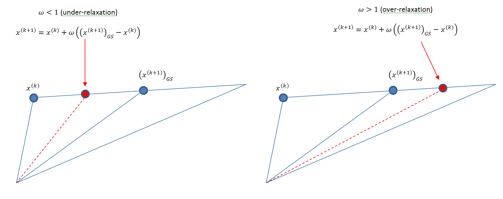
Figure 1. Illustration of under- and over-relaxation methods

Problems

Create a recursive function in Mathematica that calculates the determinant and compare it with the built-in determinant function. Test your function on matrices in $\mathbb{M}^n$ for $n=2,3,4,5,6$ , and $7$ .
Use Cramer’s rule to solve the linear system of equations $Ax=b$ defined as:
$\left(\begin{matrix}1&2&3&7\\2&3&4&8\\-1&2&3&1\\4&5&6&1\end{matrix}\right)\left(\begin{array}{c}x_1\\x_2\\x_3\\x_4\end{array}\right)=\left(\begin{array}{c}3\\2\\4\\7\end{array}\right)$
Use the naive Gauss elimination method to solve the linear system of equations $Ax=b$ defined as:
$\left(\begin{matrix}1&2&3&7\\2&3&4&8\\-1&2&3&1\\4&5&6&1\end{matrix}\right)\left(\begin{array}{c}x_1\\x_2\\x_3\\x_4\end{array}\right)=\left(\begin{array}{c}3\\2\\4\\7\end{array}\right)$
Use the Cramer’s rule code, the naive Gauss elimination method code, and the Gauss-Jordan elimination method code given above to test how many “simple” equations the algorithm can solve in less than a minute for each method. You can do so by constructing the identity matrix of dimension $n$ (using the command IdentityMatrix[n]) and a vector of values 1 of dimension $n$ and then running the code. The solution to this should be $\forall i:x_i=1$ . Repeat for higher values of $n$ . If you surround your code with the command Timing[] it should give you an indication of how long the computations are taking. Draw the curve between the size of the system $n$ and the timing taken by each method to find the solution. Is the relationship between the time taken to solve the system of equations and the size of the matrix linear or nonlinear?
Repeat problem 4, however, in this case, use the commands:
```
A = RandomReal[{-1, 1}, {n, n}];
b = RandomReal[{-1, 1}, n];
```
to generate a matrix $A$ that is $n\times n$ with random coefficients between -1 and 1 and a vector $b$ with random numbers between -1 and 1. Does this affect the results of the time taken to solve the system as a function of the matrix size and the method used?
Using random numbers similar to the previous problem, draw the curve showing the time taken to solve the system of equations as a function of the matrix size. Compare the LU decomposition, the naive Gauss elimination, and the Gauss-Jordan method. Try to optimize the code of the three methods and see if the generated curves are affected.
Calculate the Cholesky Decomposition for the following positive definite symmetric matrix:
$A= \left(\begin{matrix}6&15&55\\15&55&225\\55&225&979\end{matrix}\right)$
Calculate the Cholesky Decomposition for the following positive definite symmetric matrix:
$A= \left(\begin{matrix}8&20&15\\20&80&50\\15&50&60\end{matrix}\right)$

Employ the results to find the solution to the system of equations:

$Ax=b=\left(\begin{array}{c}50\\250\\100\end{array}\right)$
Find the LU factorization of the following matrix:
$A=\left(\begin{matrix}10&2&-1\\-3&-6&2\\1&1&5 \end{matrix}\right)$

Employ the results to find two solutions for the vector $x$ corresponding to the following two linear systems of equations:

$\begin{split} Ax&=b=\left(\begin{array}{c}12\\18\\-6\end{array}\right)\\ Ax&=b=\left(\begin{array}{c}27\\-61.5\\-21.5\end{array}\right) \end{split}$
Using the “Timing” keyword in Mathematica, compare the efficiency of the Cholesky Decomposition code provided above in comparison the built-in “CholeskyDecomposition” function in Mathematica by finding the decomposition for the identity matrix of size $n$ . Can you produce a more efficient version of the provided code?
Use the “CholeskyDecomposition” built-in function in Mathematica to produce a code to utilize the Cholesky Decomposition method to solve the linear system $Ax=b$ when $A$ is positive definite symmetric matrix. Compare with the Gauss elimination, the Gauss-Jordan elimination and the LU decomposition methods when solving the simple system of equations $Ix=b$ where $b$ is a vector whose components are all equal to 1. Similar to problem 4, draw the relationship showing the timing as a function of the size of the matrix $n$ .
Use Mathematica to program the Jacobi method such that the code would re-arrange the rows of the matrix $A$ to ensure that the diagonal entries are all non-zero.
Compare the Jacobi method and the Gauss elimination method to solve the simple system of equations $Ix=b$ where $b$ is a vector whose components are all equal to 5. Similar to problem 4, draw the relationship showing the timing as a function of the size of the matrix $n$ . What do you notice about the Jacobi method in this case?
Use the Gauss-Seidel method to find a solution to the following system after converting it into a diagonally dominant system:
$\begin{split} x_1+3x_2-x_3&=5\\ 3x_1-x_2&=5\\ x_2+2x_3&=1 \end{split}$
The following system is not diagonally dominant. Check whether the Jacobi and Gauss-Seidel methods converge or not using an initial guess of the zero vector.
$\begin{split} 4x_1+2x_2-2x_3&=0\\ x_1-3x_2-x_3&=7\\ 3x_1-x_2+4x_3&=5 \end{split}$
Assuming a stopping criterion of $\varepsilon_s=0.000001$ , find the optimal value of $\omega$ in the SOR method producing the fastest convergence in finding the solution to the following system. Compare with the Gauss-Seidel method.
$\begin{split} 4x_1+3x_2&=24\\ 3x_1+4x_2-x_3&=30\\ -x_2+4x_3&=-24 \end{split}$
Use the Gauss-Seidel method with $\varepsilon_s=0.005$ to solve the following system of linear equations:
$\begin{split} 15c_1-3c_2-c_3=3800\\ -3c_1+18c_2-6c_3=1200\\ -4c_1-c_2+12c_3=2350 \end{split}$
An electrical engineer supervises the production of three types of electrical components. Three kinds of material: metal, plastic, and rubber are required for production. The amounts needed to produce one unit of component 1 are 15 g of metal, 0.25 g of plastic, and 1.0 g of rubber. The amounts needed to produce one unit of component 2 are 17g of metal, 0.33g of plastic, and 1.2g of rubber. The amounts needed to produce one unit of component 3 are 19 g of metal, 0.42 g of plastic, and 1.6 g of rubber. If a total of 2.12, 0.0434, and 0.164 kg of metal, plastic, and rubber, respectively, are available each day. How many units of each component on average can be produced every day?
Use the Gauss-Jordan elimination method to solve the following linear system of equations:
$\begin{split} 120x_1-40x_2=637.65\\ -40x_1+110x_2-70x_3=735.75\\ -70x_2+170x_3-100x_4=588.60\\ -100x_3+120x_4-20x_5=735.75\\ -20x_4+20x_5=882.90 \end{split}$