Engineering at Alberta Courses » Finding Roots of Equations

Introduction to Numerical Analysis: Finding Roots of Equations

Let $f:[a,b]\rightarrow \mathbb{R}$ be a function. One of the most basic problems in numerical analysis is to find the value $x\in[a,b]$ that would render $f(x)=0$ . This value $x$ is called a root of the equation $f$ . As an example, consider the function $f(x)=2x-20$ . Consider the equation $f(x)=0$ . Clearly, there is only one root to this equation which is $x=10$ . Alternatively, consider $g:\mathbb{R}\rightarrow\mathbb{R}$ defined as $g(x)=a\times x^2+b\times x+c$ with $a,b,c\in\mathbb{R}$ . There are two analytical roots for the equation $g(x)=0$ given by

$x=\frac{-b\pm \sqrt{b^2-4ac}}{2a}$

In this section we are going to present three classes of methods: graphical, bracketing, and open methods for finding roots of equations.

Graphical Methods

Graphical methods rely on a computational device that calculates the values of the function along an interval at specific steps, and then draws the graph of the function. By visual inspection, the analyst can identify the points at which the function crosses the $x$ axis. Graphical methods are very useful for one-dimensional problems, but for multi-dimensional problems it is not possible to visualize a graph of a function of multi-variables.

Example

As an example, consider $f(x)=\sin{5x}+\cos{2x}$ . We wish to find the values of $x$ (i.e., the roots) that would satisfy the equation $f(x)=0$ for $x\in[-1,1]$ . The fastest way is to plot the graph (even Microsoft Excel would serve as an appropriate tool here) and then visually inspect the locations where the graph crosses the $x$ axis:

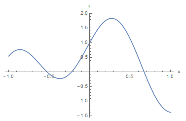
As shown in the above graph, the equation has three roots and just by visual inspection, the roots are around $x_1=-0.525$ , $x_2=-0.21$ , and $x_3=0.675$ . Of course these estimates are not that accurate for $f(x_1)=0.00365$ , $f(x_2)=0.0457$ , and $f(x_3)=-0.012$ . Whether these estimates are acceptable or not, depends on the requirements of the problem. We can further zoom in using the software to try and get better estimates:

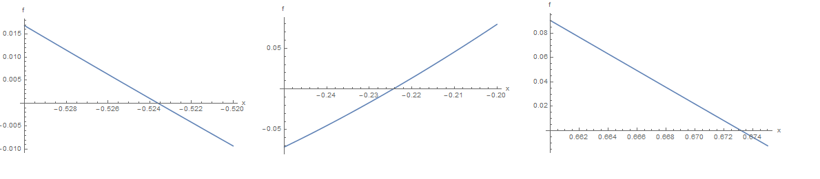
Visual inspection of the zoomed-in graphs provides the following estimates: $x_1=-0.5235$ , $x_2=-0.225$ , and $x_3=0.6731$ which are much better estimates since: $f(x_1)=0.00025$ , $f(x_2)=-0.0018$ , and $f(x_3)=0.00067$

View Mathematica Code

Clear[x]
f = Sin[5 x] + Cos[2 x]
Plot[f, {x, -1, 1}, AxesLabel -> {"x", "f"}]
f /. x -> -0.525
f /. x -> -0.21
f /. x -> 0.675
Plot[f, {x, -0.53, -0.52}, AxesLabel -> {"x", "f"}]
Plot[f, {x, -0.25, -0.2}, AxesLabel -> {"x", "f"}]
Plot[f, {x, 0.66, 0.675}, AxesLabel -> {"x", "f"}]
f /. x -> -0.5235
f /. x -> -0.225
f /. x -> 0.6731

Bracketing Methods

An elementary observation from the previous method is that in most cases, the function changes signs around the roots of an equation. The bracketing methods rely on the intermediate value theorem.

Intermediate Value Theorem

Statement: Let $f:[a,b]\rightarrow \mathbb{R}$ be continuous and $f(a)\leq f(b)$ . Then, $\forall y\in[f(a),f(b)]:\exists x\in[a,b]$ such that $y=f(x)$ . The same applies if $f(b)\leq f(a)$ .
The proof for the intermediate value theorem relies on the assumption of continuity of the function $f$ . Intuitively, because the function $f$ is continuous, then for the values of $f$ to change from $f(a)$ to $f(b)$ it has to pass by every possible value between $f(a)$ and $f(b)$ . The consequence of the theorem is that if the function $f$ is such that $f(a)\leq 0 \leq f(b)$ , then, there is $x\in[a,b]$ such that $f(x)=0$ . We can proceed to find $x$ iteratively using either the bisection method or the false position method.

Bisection Method

In the bisection method, if $f(a)f(b)<0$ , an estimate for the root of the equation $f(x)=0$ can be found as the average of $a$ and $b$ :

$x_i=\frac{a+b}{2}$

Upon evaluating $f(x_i)$ , the next iteration would be to set either $a=x_i$ or $b=x_i$ such that for the next iteration the root $x_{i+1}$ is between $a$ and $b$ . The following describes an algorithm for the bisection method given $a<b$ , $f(x)$ , $\varepsilon_s$ , and maximum number of iterations:
Step 1: Evaluate $f(a)$ and $f(b)$ to ensure that $f(a)f(b)<0$ . Otherwise, exit with an error.
Step 2: Calculate the value of the root in iteration $i$ as $x_i=\frac{a_i+b_i}{2}$ . Check which of the following applies:

If $f(x_i)=0$ , then the root has been found, the value of the error $\varepsilon_r=0$ . Exit.
If $f(x_i)f(a_i)<0$ , then for the next iteration, $x_{i+1}$ is bracketed between $a_i$ and $x_i$ . The value of $\varepsilon_r=\frac{x_{i+1}-x_{i}}{x_{i+1}}$ .
If $f(x_i)f(b_i)<0$ , then for the next iteration, $x_{i+1}$ is bracketed between $x_i$ and $b_i$ . The value of $\varepsilon_r=\frac{x_{i+1}-x_{i}}{x_{i+1}}$ .

Step 3: Set $i=i+1$ . If $i$ reaches the maximum number of iterations or if $\varepsilon_r\leq \varepsilon_s$ , then the iterations are stopped. Otherwise, return to step 2 with the new interval $a_{i+1}$ and $b_{i+1}$ .

Example

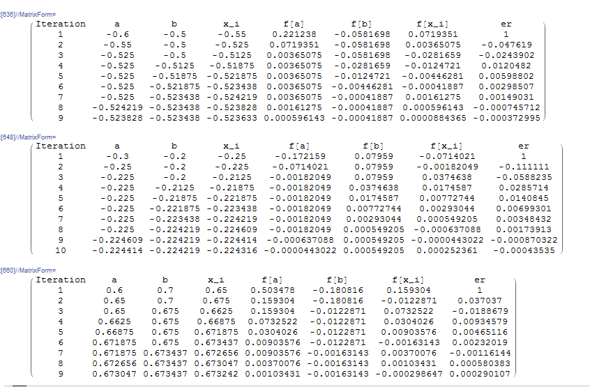
Setting $\varepsilon_s=0.0005$ and applying this process to $f(x)=\sin{5x}+\cos{2x}$ with $a=-0.6$ and $b=-0.5$ yields the estimate $x_9=-0.523633$ after 9 iterations with $\varepsilon_r=-0.000373$ as shown below. Similarly, applying this process to $f(x)=\sin{5x}+\cos{2x}$ with $a=-0.3$ and $b=-0.2$ yields the estimate $x_{10}=-0.224316$ after 10 iterations with $\varepsilon_r=-0.000435$ while applying this process to $f(x)=\sin{5x}+\cos{2x}$ with $a=0.6$ and $b=0.7$ yields the estimate $x_9=0.673242$ after 9 iterations with $\varepsilon_r=0.00029$ :

Bisection1

View Mathematica Code

Clear[f, x, ErrorTable, ei]
f[x_] := Sin[5 x] + Cos[2 x]
(*The following function returns x_i and the new interval (a,b) along with an error note. The order of the output is {xi,new a, new b, note}*)
bisec2[f_, a_, b_] := (xi = (a + b)/2; Which[
   f[a]*f[b] > 0, {xi, a, b, "Root Not Bracketed"},
   f[xi] == 0, {xi, a, b, "Root Found"},
   f[xi]*f[a] < 0, {xi, a, xi, "Root between a and xi"},
   f[xi]*f[b] < 0, {xi, xi, b, "Root between xi and b"}])


(*Problem Setup*)
MaxIter = 20;
eps = 0.0005;

(*First root*)
ErrorTable = {1};
ErrorNoteTable = {};
atable = {-0.6};
btable = {-0.5};
xtable = {};
i = 1;
Stopcode = "NoStopping";


While[And[i <= MaxIter, Stopcode == "NoStopping"],
 ri = bisec2[f, atable[[i]], btable[[i]]];
 If[ri[[4]] == "Root Not Bracketed", xtable = Append[xtable, ri[[1]]];ErrorNoteTable = Append[ErrorNoteTable, ri[[4]]]; Break[]];
 If[ri[[4]] == "Root Found", xtable = Append[xtable, ri[[1]]]; ErrorTable = Append[ErrorTable, 0];ErrorNoteTable = Append[ErrorNoteTable, ri[[4]]]; Break[]];
 atable = Append[atable, ri[[2]]];
 btable = Append[btable, ri[[3]]];
 xtable = Append[xtable, ri[[1]]];
 ErrorNoteTable = Append[ErrorNoteTable, ri[[4]]];
 If[i != 1,
  ei = (xtable[[i]] - xtable[[i - 1]])/xtable[[i]];
  ErrorTable = Append[ErrorTable, ei]];
 If[Abs[ErrorTable[[i]]] > eps, Stopcode = "NoStopping", Stopcode = "Stop"];
 i++]
Title = {"Iteration", "a", "b", "x_i", "f[a]", "f[b]", "f[x_i]", "er", "ErrorNote"};
T2 = Table[{i, atable[[i]], btable[[i]], xtable[[i]], f[atable[[i]]], f[btable[[i]]], f[xtable[[i]]], ErrorTable[[i]], ErrorNoteTable[[i]]}, {i, Length[xtable]}];
T2 = Prepend[T2, Title];
T2 // MatrixForm


(*Second Root*)
ErrorTable = {1};
ErrorNoteTable = {};
atable = {-0.3};
btable = {-0.2};
xtable = {};
i = 1;
Stopcode = "NoStopping";


While[And[i <= MaxIter, Stopcode == "NoStopping"],
 ri = bisec2[f, atable[[i]], btable[[i]]];
 If[ri[[4]] == "Root Not Bracketed", xtable = Append[xtable, ri[[1]]];ErrorNoteTable = Append[ErrorNoteTable, ri[[4]]]; Break[]];
 If[ri[[4]] == "Root Found", xtable = Append[xtable, ri[[1]]]; ErrorTable = Append[ErrorTable, 0];ErrorNoteTable = Append[ErrorNoteTable, ri[[4]]]; Break[]];
 atable = Append[atable, ri[[2]]];
 btable = Append[btable, ri[[3]]];
 xtable = Append[xtable, ri[[1]]];
 ErrorNoteTable = Append[ErrorNoteTable, ri[[4]]];
 If[i != 1,
  ei = (xtable[[i]] - xtable[[i - 1]])/xtable[[i]];
  ErrorTable = Append[ErrorTable, ei]];
 If[Abs[ErrorTable[[i]]] > eps, Stopcode = "NoStopping", Stopcode = "Stop"];
 i++]
Title = {"Iteration", "a", "b", "x_i", "f[a]", "f[b]", "f[x_i]", "er", "ErrorNote"};
T2 = Table[{i, atable[[i]], btable[[i]], xtable[[i]], f[atable[[i]]], f[btable[[i]]], f[xtable[[i]]], ErrorTable[[i]], ErrorNoteTable[[i]]}, {i, Length[xtable]}];
T2 = Prepend[T2, Title];
T2 // MatrixForm

(*Third Root*)
ErrorTable = {1};
ErrorNoteTable = {};
atable = {0.6};
btable = {0.7};
xtable = {};
i = 1;
Stopcode = "NoStopping";


While[And[i <= MaxIter, Stopcode == "NoStopping"],
 ri = bisec2[f, atable[[i]], btable[[i]]];
 If[ri[[4]] == "Root Not Bracketed", xtable = Append[xtable, ri[[1]]];ErrorNoteTable = Append[ErrorNoteTable, ri[[4]]]; Break[]];
 If[ri[[4]] == "Root Found", xtable = Append[xtable, ri[[1]]]; ErrorTable = Append[ErrorTable, 0];ErrorNoteTable = Append[ErrorNoteTable, ri[[4]]]; Break[]];
 atable = Append[atable, ri[[2]]];
 btable = Append[btable, ri[[3]]];
 xtable = Append[xtable, ri[[1]]];
 ErrorNoteTable = Append[ErrorNoteTable, ri[[4]]];
 If[i != 1,
  ei = (xtable[[i]] - xtable[[i - 1]])/xtable[[i]];
  ErrorTable = Append[ErrorTable, ei]];
 If[Abs[ErrorTable[[i]]] > eps, Stopcode = "NoStopping", Stopcode = "Stop"];
 i++]
Title = {"Iteration", "a", "b", "x_i", "f[a]", "f[b]", "f[x_i]", "er", "ErrorNote"};
T2 = Table[{i, atable[[i]], btable[[i]], xtable[[i]], f[atable[[i]]], f[btable[[i]]], f[xtable[[i]]], ErrorTable[[i]], ErrorNoteTable[[i]]}, {i, Length[xtable]}];
T2 = Prepend[T2, Title];
T2 // MatrixForm

The following code can be used to implement the bisection method in MATLAB. For the sake of demonstration, it finds the roots of the function in above example. The example function is defined in another file

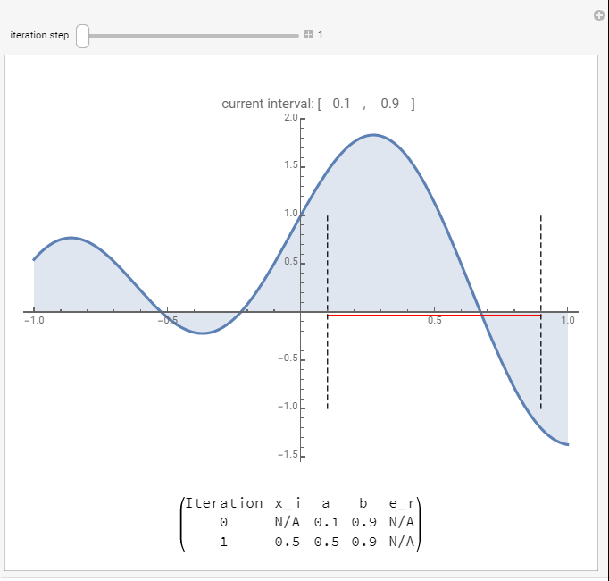
MATLAB file for the main script Download

MATLAB file for the example function Download

The following tool illustrates this process for $a=0.1$ and $b=0.9$ . Use the slider to view the process after each iteration. In the first iteration, the interval $[a,b]=[0.1,0.9]$ . $f(a)f(b)<0$ , so, $x_1=\frac{a+b}{2}=0.5$ . In the second iteration, the interval becomes $[0.5,0.9]$ and the new estimate $x_2=\frac{0.5+0.9}{2}=0.7$ . The relative approximate error in the estimate $\varepsilon_r=\frac{0.7-0.5}{0.7}=0.2857$ . You can view the process to see how it converges after 12 iterations.

Error Estimation

If $V_t$ is the true value of the root and $V_a$ is the estimate, then, the number of iterations $n$ needed to ensure that the absolute value of the error $|E|=|V_t-V_a|$ is less than or equal to a certain value can be easily obtained. Let $L=b-a$ be the length of the original interval used. The first estimate $x_1=\frac{a+b}{2}$ and so, in the next iteration, the interval where the root is contained has a length of $\frac{L}{2}$ . As the process evolves, the interval for the iteration number $n$ has a length of $\frac{L}{2^n}$ . Since the true value exists in an interval of length $\frac{L}{2^n}$ , the absolute value of the error is such that:

$|E|\leq \frac{L}{2^n}$

Therefore, for a desired estimate of the absolute value of the error, say $E_{max}$ , the number of iterations required is:

$\frac{L}{2^n}=E_{max}\Rightarrow n=\frac{\ln{\frac{L}{E_{max}}}}{\ln{2}}$

Example

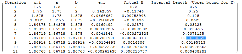
As an example, consider $f(x)=x^3+x^2-10$ , if we wish to find the root of the equation $f(x)=0$ in the interval $[1,2]$ with an absolute error less than or equal to 0.004, the number of iterations required is 8:

$n=\frac{\ln{\frac{1}{0.004}}}{\ln{2}}= 7.966 \approx 8$

The actual root with 10 significant digits is $V_t=1.867460025$ .
Using the process above, after the first iteration, $x_1=1.5$ and so, the root lies between $1.5$ and $2$ . So, the length of the interval is equal to 0.5 and the error in the estimate is less than 0.5. The length of the interval after iteration 8 is equal to 0.0039 and so the error in the estimate is less than 0.0039. It should be noted however that the actual error was less than this upper bound after the seventh iteration.
table111

View Mathematica Code

Clear[f, x, tt, ErrorTable, nn];
f[x_] := x^3 + x^2 - 10;
bisec[f_, a_, b_] := If[f[a] f[b] <= 0, If[f[(a + b)/2] f[a] <= 0, {(a + b)/2, a, (a + b)/2}, If[f[(a + b)/2] f[b] <= 0, {(a + b)/2, (a + b)/2, b}]], "Error, root is not bracketed"];
(*Exact Solution*)
t = Solve[x^3 + x^2 - 10 == 0, x]
Vt = N[x /. t[[1]], 10]

(*Problem Setup*)
MaxIter = 20;
eps = 0.0005;

(*First root*)
x = {bisec[f, 1., 2]};
ErrorTable = {1};
ErrorTable2 = {"N/A"};
IntervalLength = {0.5};
i = 2;
While[And[i <= MaxIter, Abs[ErrorTable[[i - 1]]] > eps], 
ri = bisec[f, x[[i - 1, 2]], x[[i - 1, 3]]];
If[ri=="Error, root is not bracketed",ErrorTable[[1]]="Error, root is not bracketed";Break[]];
x = Append[x, ri]; ei = (x[[i, 1]] - x[[i - 1, 1]])/x[[i, 1]]; e2i = x[[i, 1]] - Vt; ErrorTable = Append[ErrorTable, ei]; IntervalLength = Append[IntervalLength, (x[[i - 1, 3]] - x[[i - 1, 2]])/2]; ErrorTable2 = Append[ErrorTable2, e2i]; i++]
x // MatrixForm
ErrorTable // MatrixForm
Title = {"Iteration", "x_i", "a", "b", "e_r", "Actual E", "Interval Length (Upper bound for E)"};
T2 = Table[{i, x[[i, 1]], x[[i, 2]], x[[i, 3]], ErrorTable[[i]], ErrorTable2[[i]], IntervalLength[[i]]}, {i, 1, Length[x]}];
T2 = Prepend[T2, Title];
T2 // MatrixForm

The procedure for solving the above example in MATLAB is available in the following files. The polynomial function is defined in a separate file.

MATLAB file for the main script Download

MATLAB file for the example polynomial function Download

False Position Method

In the false position method, the new estimate $x_i$ at iteration $i$ is obtained by considering the linear function passing through the two points $(a,f(a))$ and $(b,f(b))$ . The point of intersection of this line with the $x$ axis can be obtained using one of the following formulas:

$x_i=a-f(a)\frac{(b-a)}{f(b)-f(a)}=b-f(b)\frac{(b-a)}{f(b)-f(a)}=\frac{af(b)-bf(a)}{f(b)-f(a)}$

Upon evaluating $f(x_i)$ , the next iteration would be to set either $a=x_i$ or $b=x_i$ such that for the next iteration the root $x_{i+1}$ is between $a$ and $b$ . The following describes an algorithm for the false position method method given $a<b$ , $f(x)$ , “varepsilon_2”, and maximum number of iterations:
Step 1: Evaluate $f(a)$ and $f(b)$ to ensure that $f(a)f(b)<0$ . Otherwise exit with an error.
Step 2: Calculate the value of the root in iteration $i$ as $x_i=\frac{a_if(b_i)-bf(a_i)}{f(b_i)-f(a_i)}$ . Check which of the following applies:

If $f(x_i)=0$ , then the root has been found, the value of the error $\varepsilon_r=0$ . Exit.
If $f(x_i)f(a_i)<0$ , then for the next iteration, $x_{i+1}$ is bracketed between $a_i$ and $x_i$ . The value of $\varepsilon_r=\frac{x_{i+1}-x_{i}}{x_{i+1}}$ .
If $f(x_i)f(b_i)<0$ , then for the next iteration, $x_{i+1}$ is bracketed between $x_i$ and $b_i$ . The value of $\varepsilon_r=\frac{x_{i+1}-x_{i}}{x_{i+1}}$ .

Step 3: If $i$ reaches the maximum number of iterations or if $\varepsilon_r\leq \varepsilon_s$ , then the iterations are stopped. Otherwise, return to step 2.

Example

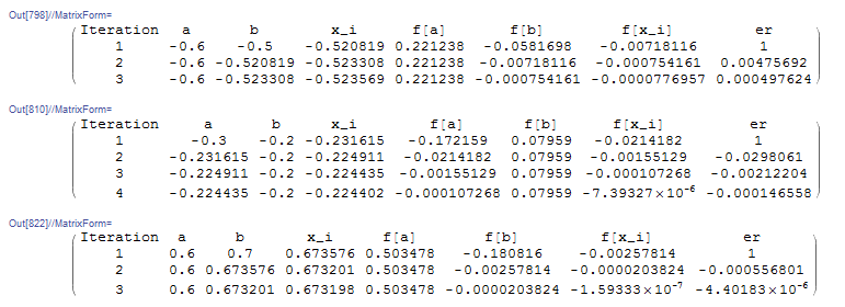
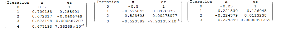
Setting $\varepsilon_s=0.0005$ and applying this process to $f(x)=\sin{5x}+\cos{2x}$ with $a=-0.6$ and $b=-0.5$ yields the estimate $x_3=-0.523569$ after 3 iterations with $\varepsilon_r=0.000498$ as shown below. Similarly, applying this process to $f(x)=\sin{5x}+\cos{2x}$ with $a=-0.3$ and $b=-0.2$ yields the estimate $x_4=-0.2244$ after 4 iterations with $\varepsilon_r=-0.00015$ while applying this process to $f(x)=\sin{5x}+\cos{2x}$ with $a=0.6$ and $b=0.7$ yields the estimate $x_3=0.673198$ after 3 iterations with $\varepsilon_r=-4.4\times 10^{-6}$ :

falseposition1

View Mathematica Code

Clear[f, x, ErrorTable, ei]
f[x_] := Sin[5 x] + Cos[2 x]
(*The following function returns x_i and the new interval (a,b) along with an error note. The order of the output is {xi,new a, new b, note}*)
falseposition[f_, a_, b_] := (xi = (a*f[b]-b*f[a])/(f[b]-f[a]); Which[
   f[a]*f[b] > 0, {xi, a, b, "Root Not Bracketed"},
   f[xi] == 0, {xi, a, b, "Root Found"},
   f[xi]*f[a] < 0, {xi, a, xi, "Root between a and xi"},
   f[xi]*f[b] < 0, {xi, xi, b, "Root between xi and b"}])


(*Problem Setup*)
MaxIter = 20;
eps = 0.0005;

(*First root*)
ErrorTable = {1};
ErrorNoteTable = {};
atable = {-0.6};
btable = {-0.5};
xtable = {};
i = 1;
Stopcode = "NoStopping";


While[And[i <= MaxIter, Stopcode == "NoStopping"],
 ri = falseposition[f, atable[[i]], btable[[i]]];
 If[ri[[4]] == "Root Not Bracketed", xtable = Append[xtable, ri[[1]]];ErrorNoteTable = Append[ErrorNoteTable, ri[[4]]]; Break[]];
 If[ri[[4]] == "Root Found", xtable = Append[xtable, ri[[1]]]; ErrorTable = Append[ErrorTable, 0];ErrorNoteTable = Append[ErrorNoteTable, ri[[4]]]; Break[]];
 atable = Append[atable, ri[[2]]];
 btable = Append[btable, ri[[3]]];
 xtable = Append[xtable, ri[[1]]];
 ErrorNoteTable = Append[ErrorNoteTable, ri[[4]]];
 If[i != 1,
  ei = (xtable[[i]] - xtable[[i - 1]])/xtable[[i]];
  ErrorTable = Append[ErrorTable, ei]];
 If[Abs[ErrorTable[[i]]] > eps, Stopcode = "NoStopping", Stopcode = "Stop"];
 i++]
Title = {"Iteration", "a", "b", "x_i", "f[a]", "f[b]", "f[x_i]", "er", "ErrorNote"};
T2 = Table[{i, atable[[i]], btable[[i]], xtable[[i]], f[atable[[i]]], f[btable[[i]]], f[xtable[[i]]], ErrorTable[[i]], ErrorNoteTable[[i]]}, {i, Length[xtable]}];
T2 = Prepend[T2, Title];
T2 // MatrixForm


(*Second Root*)
ErrorTable = {1};
ErrorNoteTable = {};
atable = {-0.3};
btable = {-0.2};
xtable = {};
i = 1;
Stopcode = "NoStopping";


While[And[i <= MaxIter, Stopcode == "NoStopping"],
 ri = falseposition[f, atable[[i]], btable[[i]]];
 If[ri[[4]] == "Root Not Bracketed", xtable = Append[xtable, ri[[1]]];ErrorNoteTable = Append[ErrorNoteTable, ri[[4]]]; Break[]];
 If[ri[[4]] == "Root Found", xtable = Append[xtable, ri[[1]]]; ErrorTable = Append[ErrorTable, 0];ErrorNoteTable = Append[ErrorNoteTable, ri[[4]]]; Break[]];
 atable = Append[atable, ri[[2]]];
 btable = Append[btable, ri[[3]]];
 xtable = Append[xtable, ri[[1]]];
 ErrorNoteTable = Append[ErrorNoteTable, ri[[4]]];
 If[i != 1,
  ei = (xtable[[i]] - xtable[[i - 1]])/xtable[[i]];
  ErrorTable = Append[ErrorTable, ei]];
 If[Abs[ErrorTable[[i]]] > eps, Stopcode = "NoStopping", Stopcode = "Stop"];
 i++]
Title = {"Iteration", "a", "b", "x_i", "f[a]", "f[b]", "f[x_i]", "er", "ErrorNote"};
T2 = Table[{i, atable[[i]], btable[[i]], xtable[[i]], f[atable[[i]]], f[btable[[i]]], f[xtable[[i]]], ErrorTable[[i]], ErrorNoteTable[[i]]}, {i, Length[xtable]}];
T2 = Prepend[T2, Title];
T2 // MatrixForm

(*Third Root*)
ErrorTable = {1};
ErrorNoteTable = {};
atable = {0.6};
btable = {0.7};
xtable = {};
i = 1;
Stopcode = "NoStopping";


While[And[i <= MaxIter, Stopcode == "NoStopping"],
 ri = falseposition[f, atable[[i]], btable[[i]]];
 If[ri[[4]] == "Root Not Bracketed", xtable = Append[xtable, ri[[1]]];ErrorNoteTable = Append[ErrorNoteTable, ri[[4]]]; Break[]];
 If[ri[[4]] == "Root Found", xtable = Append[xtable, ri[[1]]]; ErrorTable = Append[ErrorTable, 0];ErrorNoteTable = Append[ErrorNoteTable, ri[[4]]]; Break[]];
 atable = Append[atable, ri[[2]]];
 btable = Append[btable, ri[[3]]];
 xtable = Append[xtable, ri[[1]]];
 ErrorNoteTable = Append[ErrorNoteTable, ri[[4]]];
 If[i != 1,
  ei = (xtable[[i]] - xtable[[i - 1]])/xtable[[i]];
  ErrorTable = Append[ErrorTable, ei]];
 If[Abs[ErrorTable[[i]]] > eps, Stopcode = "NoStopping", Stopcode = "Stop"];
 i++]
Title = {"Iteration", "a", "b", "x_i", "f[a]", "f[b]", "f[x_i]", "er", "ErrorNote"};
T2 = Table[{i, atable[[i]], btable[[i]], xtable[[i]], f[atable[[i]]], f[btable[[i]]], f[xtable[[i]]], ErrorTable[[i]], ErrorNoteTable[[i]]}, {i, Length[xtable]}];
T2 = Prepend[T2, Title];
T2 // MatrixForm

The procedure for implementing the false position root finding algorithm in MATLAB is available in the following files. The example function is defined in a separate file.

MATLAB file for the main script Download

MATLAB file for the example polynomial function Download

The following tool illustrates this process for $a=0.1$ and $b=0.9$ . Use the slider to view the process after each iteration. In the first iteration, the interval $[a,b]=[0.1,0.9]$ . $f(a)f(b)<0$ , so, $x_1=\frac{0.1f(0.9)-0.9f(0.1)}{f(0.9)-f(0.1)}=0.538249$ . In the second iteration, the interval becomes $[0.538249,0.9]$ and the new estimate $x_2=\frac{0.538249f(0.9)-0.9f(0.538249)}{f(0.9)-f(0.538249)}=0.693886$ . The relative approximate error in the estimate $\varepsilon_r=\frac{0.693886-0.538249}{0.693886}=0.224297$ . You can view the process to see how it converges after very few iterations.

Open Methods

Open methods do not rely on having the root squeezed between two values, but rather rely on an initial guess and then apply an iterative process to get better estimates for the root. Open methods are usually faster in convergence if they converge, but they don’t always converge. For multi-dimensions, i.e., for solving multiple nonlinear equations, open methods are easier to implement than bracketing methods which cannot be easily extended to multi-dimensions.

Fixed-Point Iteration Method

Let $g:V\rightarrow V$ . A fixed point of $g$ is defined as $x\in V$ such that $x=g(x)$ . If $g:\mathbb{R}\rightarrow \mathbb{R}$ , then a fixed point of $g$ is the intersection of the graphs of the two functions $f(x)=x$ and $g(x)$ .

The fixed-point iteration method relies on replacing the expression $f(x)=0$ with the expression $x=g(x)$ . Then, an initial guess for the root $x_1$ is assumed and input as an argument for the function $g$ . The output $g(x_1)$ is then the estimate $x_2$ . The process is then iterated until the output $x_{n+1}\approx g(x_n)$ . The following is the algorithm for the fixed-point iteration method. Assuming $x_0$ , $\varepsilon_s$ , and maximum number of iterations $N$ :
Set $x_{n+1}=g(x_n)$ , and calculate $\varepsilon_r=\frac{x_{n+1}-x_{n}}{x_{n+1}}$ and compare with $\varepsilon_s$ . If $|\varepsilon_r|\leq \varepsilon_s$ or if $n=N$ , then stop the procedure, otherwise, repeat.

The Babylonian method for finding roots described in the introduction section is a prime example of the use of this method. If we seek to find the solution for the equation $x^2=s$ or $f(x)=x^2-s=0$ , then a fixed-point iteration scheme can be implemented by writing this equation in the form:

$x=\frac{x+\frac{s}{x}}{2}$

Example

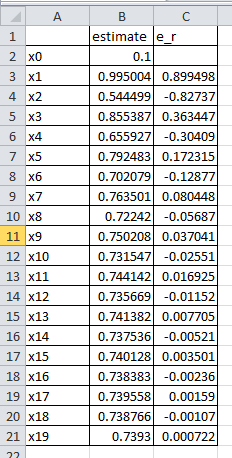
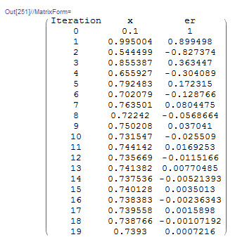
Consider the function $f(x)=\cos{x}-x$ . We wish to find the root of the equation $f(x)=0$ , i.e., $\cos{x}-x=0$ . The expression can be rearranged to the fixed-point iteration form $x=\cos{x}$ and an initial guess $x_0=0.1$ can be used. The tolerance $\varepsilon_s$ is set to 0.001. The following is the Microsoft Excel table showing that the tolerance is achieved after 19 iterations:
excel1

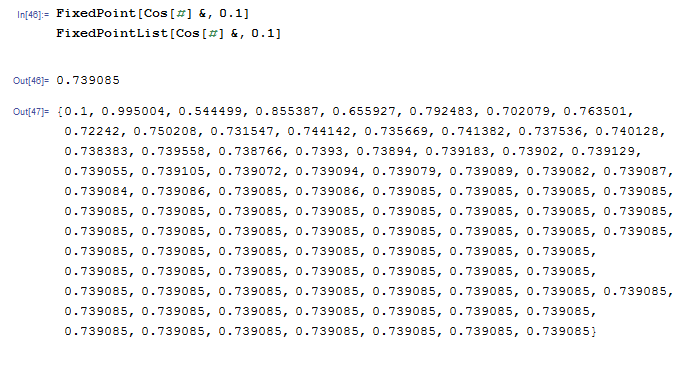
Mathematica has a built-in algorithm for the fixed-point iteration method. The function “FixedPoint[f,Expr,n]” applies the fixed-point iteration method $x=f(x)$ with the initial guess being “Expr” with a maximum number of iterations “n”. As well, the function “FixedPointList[f,Expr,n]” returns the list of applying the function “n” times. If “n” is omitted, then the software applies the fixed-point iteration method until convergence is achieved. Here is a snapshot of the code and the output for the fixed-point iteration $x=\cos{x}$ . The software finds the solution $x=0.739085$ . Compare the list below with the Microsoft Excel sheet above.
fixedpoint1

Alternatively, simple code can be written in Mathematica with the following output
fixedpoint2
View Mathematica Code

x = {0.1};
er = {1};
es = 0.001;
MaxIter = 100;
i = 1;
While[And[i <= MaxIter, Abs[er[[i]]] > es],  xnew = Cos[x[[i]]]; x = Append[x, xnew]; ernew = (xnew - x[[i]])/xnew; er = Append[er, ernew]; i++];
T = Length[x];
SolutionTable = Table[{i - 1, x[[i]], er[[i]]}, {i, 1, T}];
SolutionTable1 = {"Iteration", "x", "er"};
T = Prepend[SolutionTable, SolutionTable1];
T // MatrixForm

The following MATLAB code runs the fixed-point iteration method to find the root of a function $f(x)$ with initial guess $x_0$ . The value of the estimate and approximate relative error at each iteration is displayed in the command window. Additionally, two plots are produced to visualize how the iterations and the errors progress. Your function should be written in the form $x = g(x)$ . Then call the fixed point iteration function with fixedpointfun2(@(x) g(x), x0). For example, try fixedpointfun2(@(x) cos(x), 0.1)

MATLAB file Download

Convergence

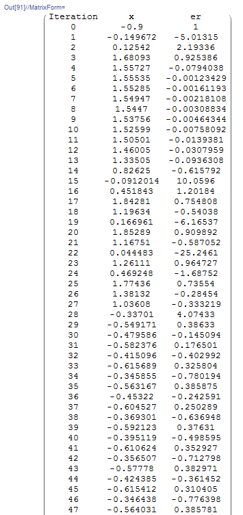
The fixed-point iteration method converges easily if in the region of interest we have $|g'(x)|<1$ . Otherwise, it does not converge. Here is an example where the fixed-point iteration method fails to converge.

Example

Consider the function $f(x)=\sin{5x}+\cos{2x}$ . To find the root of the equation $f(x)=0$ , the expression can be converted into the fixed-point iteration form as:
$x=\sin{5x}+\cos{2x}+x$ . Implementing the fixed-point iteration procedure shows that this expression almost never converges but oscillates:

View Mathematica Code

Clear[x, g]
x = {-0.9};
er = {1};
es = 0.001;
MaxIter = 100;
i = 1;
g[x_] := (Sin[5 x] + Cos[2 x]) + x
While[And[i <= MaxIter, Abs[er[[i]]] > es],xnew = g[x[[i]]]; x = Append[x, xnew]; ernew = (xnew - x[[i]])/xnew;er = Append[er, ernew]; i++];
T = Length[x];
SolutionTable = Table[{i - 1, x[[i]], er[[i]]}, {i, 1, T}];
SolutionTable1 = {"Iteration", "x", "er"};
T = Prepend[SolutionTable, SolutionTable1];
T // MatrixForm

The following is the output table showing the first 45 iterations. The value of the error oscillates and never decreases:
fixedpoint3

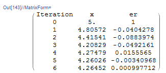
The expression $f(x)=0$ can be converted to different forms $x=g(x)$ . For example, assuming $x\neq 0$ :

$0=\sin{5x}+\cos{2x}\Rightarrow 0=\frac{\sin{5x}+\cos{2x}}{x}\Rightarrow x=\frac{\sin{5x}+\cos{2x}}{x}+x$

If this expression is used, the fixed-point iteration method does converge depending on the choice of $x_0$ . For example, setting $x_0=5.0$ gives the estimate for the root $x_6=4.26452$ with the required accuracy:
fixedpoint4

View Mathematica Code

Clear[x, g]
x = {5.};
er = {1};
es = 0.001;
MaxIter = 100;
i = 1;
g[x_] := (Sin[5 x] + Cos[2 x])/x + x
While[And[i <= MaxIter, Abs[er[[i]]] > es], xnew = g[x[[i]]]; x = Append[x, xnew]; ernew = (xnew - x[[i]])/xnew; er = Append[er, ernew]; i++];
T = Length[x];
SolutionTable = Table[{i - 1, x[[i]], er[[i]]}, {i, 1, T}];
SolutionTable1 = {"Iteration", "x", "er"};
T = Prepend[SolutionTable, SolutionTable1];
T // MatrixForm

Obviously, unlike the bracketing methods, this open method cannot find a root in a specific interval. The root is a function of the initial guess $x_0$ and the form $x=g(x)$ , but the user has no other way of forcing the root to be within a specific interval. It is very difficult, for example, to use the fixed-point iteration method to find the roots of the expression $0=\sin{5x}+\cos{2x}$ in the interval $[-1,1]$ .

Analysis of Convergence of the Fixed-Point Method

The objective of the fixed-point iteration method is to find the true value $V_t$ that satisfies $V_t=g(V_t)$ . In each iteration we have the estimate $x_{i+1}=g(x_i)$ . Using the mean value theorem, we can write the following expression:

$g(x_i)=g(V_t)+g'(\xi)(x_i-V_t)$

for some $\xi$ in the interval between $x_i$ and the true value $V_t$ . Replacing $g(V_t)$ and $g(x_i)$ in the above expression yields:

$x_{i+1}=V_t+g'(\xi)(x_i-V_t)\Rightarrow x_{i+1}-V_t=g'(\xi)(x_i-V_t)$

The error after iteration $i+1$ is equal to $E_{i+1}=V_t-x_{i+1}$ while that after iteration $i$ is equal to $E_i=V_t-x_i$ . Therefore, the above expression yields:

$E_{i+1}=g'(\xi)E_i$

For the error to reduce after each iteration, the first derivative of $g$ , namely $g'$ , should be bounded by 1 in the region of interest (around the required root):

$|g'(\xi)|< 1$

We can now try to understand why, in the previous example, the expression $x=g(x)=\sin{5x}+\cos{2x}+x$ does not converge. When we plot $g(x)$ and $g'(x)$ we see that $g'(x)$ oscillates rapidly with values higher than 1:

fixedpoint5

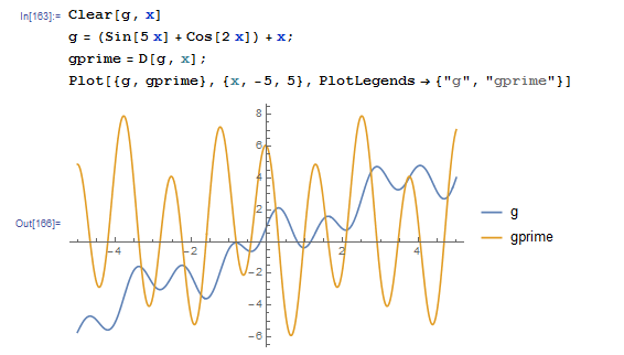
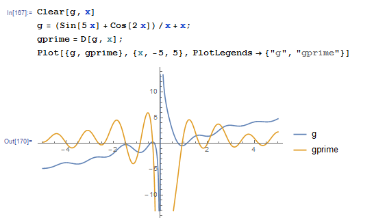
On the other hand, the expression $x=g(x)=\frac{\sin{5x}+\cos{2x}}{x}+x$ converges for roots that are away from zero. When we plot $g(x)$ and $g'(x)$ we see that the oscillations in $g'(x)$ decrease when $x$ is away from zero and $g'(x)$ is bounded by 1 in some regions:
fixedpoint6

Example

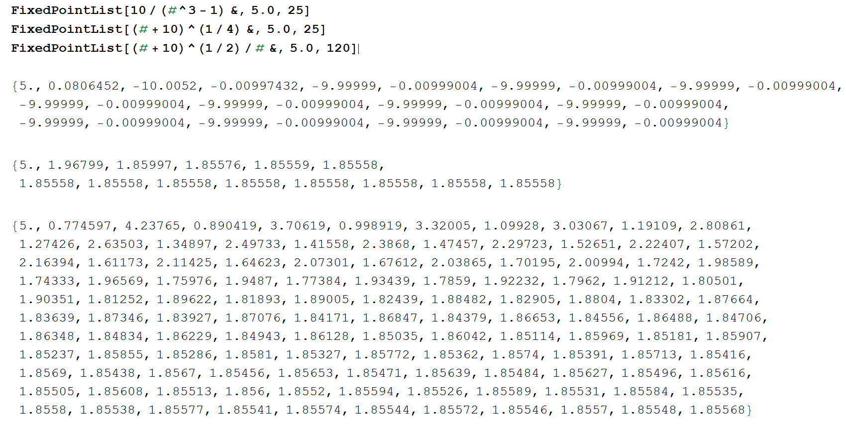
In this example, we will visualize the example of finding the root of the expression $x^4-x-10=0$ . There are three different forms for the fixed-point iteration scheme:

$\begin{split} x&=g_1(x)=\frac{10}{x^3-1}\\ x&=g_2(x)=(x+10)^{1/4}\\ x&=g_3(x)=\frac{(x+10)^{1/2}}{x} \end{split}$

To visualize the convergence, notice that if we plot the separate graphs of the function $x$ and the function $g(x)$ , then, the root is the point of intersection when $x=g(x)$ . For $g_1(x)$ , the slope $g_1'(x)$ is not bounded by 1 and so, the scheme diverges no matter what $x_0$ is. Here we start with $x_0=2$ :

For $g_2(x)$ , the slope $g_2'(x)$ is bounded by 1 and so, the scheme converges really fast no matter what $x_0$ is. Here we start with $x_0=5$ :

For $g_3(x)$ , the slope $g_3'(x)$ is bounded by 1 and so, the scheme converges but slowly. Here we start with $x_0=5$ :

The following is the Mathematica code used to generate one of the tools above:
View Mathematica Code

Manipulate[
 x = {5.};
 er = {1};
 es = 0.001;
 MaxIter = 20;
 i = 1;
 g[x_] := (x + 10)^(1/4);
 While[And[i <= MaxIter, Abs[er[[i]]] > es],xnew = g[x[[i]]]; x = Append[x, xnew]; ernew = (xnew - x[[i]])/xnew;er = Append[er, ernew]; i++];
 T1 = Length[x];
 SolutionTable = Table[{i - 1, x[[i]], er[[i]]}, {i, 1, T1}];
 SolutionTable1 = {"Iteration", "x", "er"};
 T = Prepend[SolutionTable, SolutionTable1];
 LineTable1 = Table[{{T[[i, 2]], T[[i, 2]]}, {T[[i, 2]], g[T[[i, 2]]]}}, {i, 2, n}];
 LineTable2 = Table[{{T[[i + 1, 2]], T[[i + 1, 2]]}, {T[[i, 2]], g[T[[i, 2]]]}}, {i, 2, n - 1}];
 Grid[{{Plot[{x, g[x]}, {x, 0, 5}, PlotLegends -> {"x", "g3(x)"},ImageSize -> Medium, Epilog -> {Dashed, Line[LineTable1], Line[LineTable2]}]}, {Row[{"Iteration=", n - 2, "    x_n=", T[[n, 2]], "   g(x_n)=", g[T[[n, 2]]]}]}}], {n, 2, Length[T], 1}]

The following shows the output if we use the built-in fixed-point iteration function for each of $g_1$ , $g_2$ , and $g_3$ . $g_1$ oscillates and so, it will never converge. $g_2$ converges really fast (3 to 4 iterations). $g_3$ converges really slow, taking up to 120 iterations to converge.
FixedPoint33

Newton-Raphson Method

The Newton-Raphson method is one of the most used methods of all root-finding methods. The reason for its success is that it converges very fast in most cases. In addition, it can be extended quite easily to multi-variable equations. To find the root of the equation $f(x_t)=0$ , the Newton-Raphson method depends on the Taylor Series Expansion of the function around the estimate $x_i$ to find a better estimate $x_{i+1}$ :

$f(x_{i+1})=f(x_i)+f'(x_i)(x_{i+1}-x_i)+\mathcal O (h^2)$

where $x_{i+1}$ is the estimate of the root after iteration $i+1$ and $x_i$ is the estimate at iteration $i$ . Assuming $f(x_{i+1})=0$ and rearranging:

$x_{i+1}\approx x_i-\frac{f(x_i)}{f'(x_i)}$

The procedure is as follows. Setting an initial guess $x_0$ , tolerance $\varepsilon_s$ , and maximum number of iterations $N$ :
At iteration $i$ , calculate $x_i\approx x_{i-1}-\frac{f(x_{i-1})}{f'(x_{i-1})}$ and $\varepsilon_r$ . If $\varepsilon_r\leq \varepsilon_s$ or if $i\geq N$ , stop the procedure. Otherwise repeat.
Note: unlike the previous methods, the Newton-Raphson method relies on calculating the first derivative of the function $f(x)$ . This makes the procedure very fast, however, it has two disadvantages. The first is that this procedure doesn’t work if the function $f(x)$ is not differentiable. Second, the inverse $(f'(x_{i}))^{-1}$ can be slow to calculate when dealing with multi-variable equations.

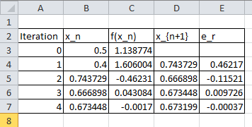
Example

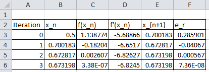
As an example, let’s consider the function $f(x)=\sin{5x}+\cos{2x}$ . The derivative of $f$ is $f'(x)=5\cos{5x}-2\sin{2x}$ . Setting the maximum number of iterations $N=100$ , $\varepsilon_s=0.0005$ , $x_0=0.5$ , the following is the Microsoft Excel table produced:
NR1

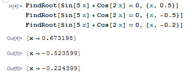
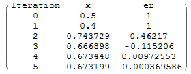
Mathematica has a built-in algorithm for the Newton-Raphson method. The function “FindRoot[lhs==rhs,{x,x0}]” applies the Newton-Raphson method with the initial guess being “x0”. The following is a screenshot of the input and output of the built-in function evaluating the roots based on three initial guesses.
NR2

Alternatively, a Mathematica code can be written to implement the Newton-Raphson method with the following output for three different initial guesses:
NR3
View Mathematica Code

Clear[x]
f[x_] := Sin[5 x] + Cos[2 x]
fp = D[f[x], x]
xtable = {-0.25};
er = {1};
es = 0.0005;
MaxIter = 100;
i = 1;
While[And[i <= MaxIter, Abs[er[[i]]] > es], xnew = xtable[[i]] - (f[xtable[[i]]]/fp /. x -> xtable[[i]]);  xtable = Append[xtable, xnew]; ernew = (xnew - xtable[[i]])/xnew;  er = Append[er, ernew]; i++];
T = Length[xtable];
SolutionTable = Table[{i - 1, xtable[[i]], er[[i]]}, {i, 1, T}];
SolutionTable1 = {"Iteration", "x", "er"};
T = Prepend[SolutionTable, SolutionTable1];
T // MatrixForm

The following MATLAB code runs the Newton-Raphson method to find the root of a function $f(x)$ with derivative $f'(x)$ and initial guess $x_0$ . The value of the estimate and approximate relative error at each iteration is displayed in the command window. Additionally, two plots are produced to visualize how the iterations and the errors progress. You need to pass the function f(x) and its derivative df(x) to the newton-raphson method along with the initial guess as newtonraphson(@(x) f(x), @(x) df(x), x0). For example, try newtonraphson(@(x) sin(5.*x)+cos(2.*x), @(x) 5.*cos(5.*x)-2.*sin(2.*x),0.4)

MATLAB file Download

Analysis of Convergence of the Newton-Raphson Method

The error in the Newton-Raphson Method can be roughly estimated as follows. The estimate $x_{i+1}$ is related to the previous estimate $x_i$ using the equation:

$x_{i+1}=x_i-\frac{f(x_i)}{f'(x_i)}\Rightarrow 0=f(x_i)+f'(x_i)(x_{i+1}-x_i)$

Additionally, using Taylor’s theorem, and if $x_t$ is the true root with $f(x_t)=0$ we have:

$f(x_t)=0=f(x_i)+f'(x_i)(x_t-x_i)+\frac{f''(\xi)}{2!}{(x_t-x_i)^2}$

for some $\xi$ in the interval between $x_i$ and $x_t$ . Subtracting the above two equations yields:

$0=f'(x_i)(x_t-x_{i+1})+\frac{f''(\xi)}{2!}{(x_t-x_i)^2}$

Since $E_{i+1}=x_t-x_{i+1}$ and $E_i=x_t-x_i$ then:

(1) $\begin{equation*} E_{i+1}=-\frac{f''(\xi)}{2!f'(x_i)}{E_i^2} \end{equation*}$

If the method is converging, we have $f''(\xi)\approx f''(x_t)$ and $f'(\xi)\approx f'(x_t)$ therefore:

$E_{i+1}\propto E_i^2$

Therefore, the error is squared after each iteration, i.e., the number of correct decimal places approximately doubles with each iteration. This behaviour is called quadratic convergence. Look at the tables in the Newton-Raphson example above and compare the relative error after each step!

The following tool can be used to visualize how the Newton-Raphson method works. Using the slope $f'(x_i)$ , the difference $x_{i+1}-x_i$ can be calculated and thus, the value of the new estimate $x_{i+1}$ can be computed accordingly. Use the slider to see how fast the method converges to the true solution using $\varepsilon_s=0.0005$ , $x_0=0.4$ , and solving for the root of $f(x)=\sin[5x]+\cos[2x]=0$ .

View Mathematica code

Manipulate[
 f[x_] := Sin[5 x] + Cos[2 x];
 fp = D[f[x], x];
 xtable = {0.4};
 er = {1};
 es = 0.0005;
 MaxIter = 100;
 i = 1;
 While[And[i <= MaxIter, Abs[er[[i]]] > es], xnew = xtable[[i]] - (f[xtable[[i]]]/fp /. x -> xtable[[i]]); xtable = Append[xtable, xnew]; ernew = (xnew - xtable[[i]])/xnew; er = Append[er, ernew]; i++];
 T = Length[xtable];
 SolutionTable = Table[{i - 1, xtable[[i]], er[[i]]}, {i, 1, T}];
 SolutionTable1 = {"Iteration", "x", "er"};
 T = Prepend[SolutionTable, SolutionTable1];
  LineTable1 = Table[{{T[[i, 2]], 0}, {T[[i, 2]], f[T[[i, 2]]]}, {T[[i + 1, 2]],0}}, {i, 2, n - 1}];
 Grid[{{Plot[f[x], {x, 0, 1}, PlotLegends -> {"f(x)"}, ImageSize -> Medium,  Epilog -> {Dashed, Line[LineTable1]}]}, {Row[{"Iteration=", n - 2, "    x_n=", T[[n, 2]], "   f(x_n)=", f[T[[n, 2]]]}]}}], {n, 2, 7, 1}]

Depending on the shape of the function and the initial guess, the Newton-Raphson method can get stuck around the locations of oscillations of the function. The tool below visualizes the algorithm when trying to find the root of $f(x)=x^3-x+3=0$ with an initial guess of $x_0=-0.1$ . It takes 33 iterations before reaching convergence.

Depending on the shape of the function and the initial guess, the Newton-Raphson method can get stuck in a loop. The tool below visualizes the algorithm when trying to find the root of $f(x)=x^3-x+3=0$ with an initial guess of $x_0=0$ . The algorithm goes into an infinite loop.

In general, an initial guess that is close enough to the true root will guarantee quick convergence. The tool below visualizes the algorithm when trying to find the root of $f(x)=x^3-x+3=0$ with an initial guess of $x_0=-1$ . The algorithm quickly converges to the desired root.

The following is the Mathematica code used to generate one of the tools above:
View Mathematica Code

Manipulate[
 f[x_] := x^3 - x + 3;
 fp = D[f[x], x];
 xtable = {-0.1};
 er = {1.};
 es = 0.0005;
 MaxIter = 100;
 i = 1;
 While[And[i <= MaxIter, Abs[er[[i]]] > es], xnew = xtable[[i]] - (f[xtable[[i]]]/fp /. x -> xtable[[i]]); xtable = Append[xtable, xnew]; ernew = (xnew - xtable[[i]])/xnew; er = Append[er, ernew]; i++];
 T = Length[xtable];
 SolutionTable = Table[{i - 1, xtable[[i]], er[[i]]}, {i, 1, T}];
 SolutionTable1 = {"Iteration", "x", "er"};
 T = Prepend[SolutionTable, SolutionTable1]; 
 LineTable1 =   Table[{{T[[i, 2]], 0}, {T[[i, 2]], f[T[[i, 2]]]}, {T[[i + 1, 2]], 0}}, {i, 2, n - 1}];
 Grid[{{Plot[f[x], {x, -3, 2}, PlotLegends -> {"f(x)"}, ImageSize -> Medium, Epilog -> {Dashed, Line[LineTable1]}]}, {Row[{"Iteration=", n - 2, "    x_n=", T[[n, 2]], "   f(x_n)=", f[T[[n, 2]]]}]}}] , {n, 2, 33, 1}]

Secant Method

The secant method is an alternative to the Newton-Raphson method by replacing the derivative $f'(x)$ with its finite-difference approximation. The secant method thus does not require the use of derivatives especially when $f(x)$ is not explicitly defined. In certain situations, the secant method is preferable over the Newton-Raphson method even though its rate of convergence is slightly less than that of the Newton-Raphson method. Consider the problem of finding the root of the function $f(x)=0$ . Starting with the Newton-Raphson equation and utilizing the following approximation for the derivative $f'(x_{i})$ :

$f'(x_i)=\frac{f(x_i)-f(x_{i-1})}{x_i-x_{i-1}}$

the estimate for iteration $i+1$ can be computed as:

$x_{i+1}=x_i-f(x_i)\frac{x_i-x_{i-1}}{f(x_i)-f(x_{i-1})}$

Obviously, the secant method requires two initial guesses $x_0$ and $x_1$ .

Example

As an example, let’s consider the function $f(x)=\sin{5x}+\cos{2x}$ . Setting the maximum number of iterations $N=100$ , $\varepsilon_s=0.0005$ , $x_0=0.5$ , and $x_1=0.4$ , the following is the Microsoft Excel table produced:
secant1

The Mathematica code below can be used to program the secant method with the following output:
secant2

View Mathematica Code

f[x_] := Sin[5 x] + Cos[2 x];
xtable = {0.5, 0.4};
er = {1,1};
es = 0.0005;
MaxIter = 100;
i = 2;
While[And[i <= MaxIter, Abs[er[[i]]] > es], xnew = xtable[[i]] - (f[xtable[[i]]]) (xtable[[i]] - xtable[[i - 1]])/(f[xtable[[i]]] -f[xtable[[i - 1]]]); xtable = Append[xtable, xnew];  ernew = (xnew - xtable[[i]])/xnew; er = Append[er, ernew]; i++];
T = Length[xtable];
SolutionTable = Table[{i - 1, xtable[[i]], er[[i]]}, {i, 1, T}];
SolutionTable1 = {"Iteration", "x", "er"};
T = Prepend[SolutionTable, SolutionTable1];
T // MatrixForm

The following code runs the Secant method to find the root of a function $f(x)$ with two initial guesses $x_0$ and $x_1$ . The value of the estimate and approximate relative error at each iteration is displayed in the command window. Additionally, two plots are produced to visualize how the iterations and the errors progress. The program waits for a keypress between each iteration to allow you to visualize the iterations in the figure. Call the function with secant(@(x) f(x), x0, x1). For example try secant(@(x) sin(5.*x)+cos(2.*x),0.5,0.4)

MATLAB file Download

Convergence Analysis of the Secant Method

The $i+1$ estimate in the secant method is obtained as follows:

$x_{i+1}=x_i-f(x_i)\frac{x_i-x_{i-1}}{f(x_i)-f(x_{i-1})}$

Multiplying both sides by -1 and adding the true value of the root $x_t$ where $f(x_t)=0$ for both sides yields:

$x_t-x_{i+1}=x_t-x_i+f(x_i)\frac{x_i-x_{i-1}}{f(x_i)-f(x_{i-1})}$

Using algebraic manipulations:

$\begin{split} x_t-x_{i+1}&=\frac{(x_t-x_i)(f(x_i)-f(x_{i-1}))+f(x_i)(x_i-x_{i-1})}{f(x_i)-f(x_{i-1})}\\ &=\frac{f(x_i)(x_t-x_{i-1})-f(x_{i-1})(x_t-x_i)}{f(x_i)-f(x_{i-1})}\\ &=(x_t-x_{i-1})(x_t-x_i)\frac{\frac{f(x_i)}{x_t-x_i}-\frac{f(x_{i-1})}{x_t-x_{i-1}}}{f(x_i)-f(x_{i-1})} \end{split}$

Using the Mean Value Theorem, the denominator on the right-hand side can be replaced with:

$f(x_i)=f(x_{i-1})+f'(\zeta)(x_i-x_{i-1})$

for some $\zeta$ between $x_i$ and $x_{i-1}$ . Therefore,

$x_t-x_{i+1}=(x_t-x_{i-1})(x_t-x_i)\frac{\frac{f(x_i)}{x_t-x_i}-\frac{f(x_{i-1})}{x_t-x_{i-1}}}{f'(\zeta)(x_i-x_{i-1})}$

Using Taylor’s theorem for $f(x_{i-1})$ and $f(x_i)$ around $x_t$ we get:

$\begin{split} \frac{f(x_i)}{x_t-x_i}=f'(x_t)+\frac{f''(\xi_1)}{2}{(x_t-x_i)}\\ \frac{f(x_i)}{x_t-x_{i-1}}=f'(x_t)+\frac{f''(\xi_2)}{2}{(x_t-x_{i-1})} \end{split}$

for some $\xi_1$ between $x_i$ and $x_t$ and some $\xi_2$ between $x_{i-1}$ and $x_t$ . Using the above expressions we can reach the equation:

$x_t-x_{i+1}=(x_t-x_{i-1})(x_t-x_i)\frac{\frac{f''(\xi_1)}{2}{(x_t-x_i)}-\frac{f''(\xi_2)}{2}{(x_t-x_{i-1})}}{f'(\zeta)(x_i-x_{i-1})}$

$\xi_1$ and $\xi_2$ can be assumed to be identical and equal to $\xi$ , therefore:

$\begin{split} x_t-x_{i+1}&=(x_t-x_{i-1})(x_t-x_i)\frac{\frac{f''(\xi)}{2}{(x_t-x_i-x_t+x_{i-1})}}{f'(\zeta)(x_i-x_{i-1})}\\ &=(x_t-x_{i-1})(x_t-x_i)\frac{-f''(\xi)}{2f'(\zeta)} \end{split}$

Therefore:

(2) $\begin{equation*} E_{i+1}=E_{i}E_{i-1}\left(\frac{-f''(\xi)}{2f'(\zeta)}\right) \end{equation*}$

Comparing 1 with 2 shows that the convergence in the secant method is not quite quadratic. To find the order of convergence, we need to solve the following equation for a positive $p$ and $C$ :

$|E_{i+1}|=C|E_{i}|^p$

Substituting into equation 2 yields:

$C|E_{i}|^p=|E_{i}||E_{i-1}|\bigg{|}\frac{-f''(\xi)}{2f'(\zeta)}\bigg{|}\Rightarrow E_{i}=\left|\frac{-f''(\xi)}{2Cf'(\zeta)}\right|^{\frac{1}{p-1}}|E_{i-1}|^{\frac{1}{p-1}}$

But we also have:

$|E_{i}|=C|E_{i-1}|^p$

Therefore: $p=\frac{1}{p-1}$ . This equation is called the golden ratio and has the positive solution for $p$ :

$p=\frac{\sqrt{5}+1}{2}\approx 1.618034$

while

$C=\left|\frac{-f''(\xi)}{2f'(\zeta)}\right|^{p-1}=\left|\frac{-f''(\xi)}{2f'(\zeta)}\right|^{0.618034}$

implying that the error convergence is not quadratic but rather:

$E_{i+1}\propto E_i^{1.618034}$

The following tool visualizes how the secant method converges to the true solution using two initial guesses. Using $\varepsilon_s=0.0005$ , $x_0=0.35$ , $x_1=0.4$ , and solving for the root of $f(x)=\sin[5x]+\cos[2x]=0$ yields $x_6=0.6732$ .

The following Mathematica Code was utilized to produce the above tool:
View Mathematica Code

Manipulate[
 f[x_] := x^3 - x + 3;
 f[x_] := Sin[5 x] + Cos[2 x];
 xtable = {-0.5, -0.6};
 xtable = {0.35, 0.4};
 er = {1, 1};
 es = 0.0005;
 MaxIter = 100;
 i = 2;
 While[And[i <= MaxIter, Abs[er[[i]]] > es], xnew = xtable[[i]] - (f[xtable[[i]]]) (xtable[[i]] - xtable[[i-1]])/(f[xtable[[i]]] -f[xtable[[i - 1]]]); xtable = Append[xtable, xnew];  ernew = (xnew - xtable[[i]])/xnew; er = Append[er, ernew]; i++];
 T = Length[xtable];
 SolutionTable = Table[{i - 1, xtable[[i]], er[[i]]}, {i, 1, T}];
 SolutionTable1 = {"Iteration", "x", "er"};
 T = Prepend[SolutionTable, SolutionTable1];
 T // MatrixForm;
 If[n > 3,
  (LineTable1 = {{T[[n - 2, 2]], 0}, {T[[n - 2, 2]], f[T[[n - 2, 2]]]}, {T[[n - 1, 2]], f[T[[n - 1, 2]]]}, {T[[n, 2]], 0}};
   LineTable2 = {{T[[n - 1, 2]], 0}, {T[[n - 1, 2]], f[T[[n - 1, 2]]]}}), LineTable1 = {{}}; LineTable2 = {{}}];
 Grid[{{Plot[f[x], {x, 0, 1}, PlotLegends -> {"f(x)"}, ImageSize -> Medium, Epilog -> {Dashed, Line[LineTable1], Line[LineTable2]}]}, {Row[{"Iteration=", n - 2, "    x_n=", T[[n, 2]], "   f(x_n)=", f[T[[n, 2]]]}]}}], {n, 2, 8, 1}]

Problems

Let $f:[-5,5]\rightarrow \mathbb{R}$ be such that $f(x)=0.5+x\cos{x}$ . Use the graphical method to find the number and estimates of the roots of each of the equations $f(x)=0$ and $f(x)=2$ .
Compare the bisection method and the false position method in finding the roots of the two equations $f(x)=0$ and $f(x)=0.1$ in the interval $[-1,1]$ where $f(x)$ is:
$f(x)=2x^3-4x^2+3x$

Compare with the result using the Solve function and comment on the use of $\varepsilon_r$ as a measure of the relative error.
Locate the first nontrivial root of $\sin{x}=x^2$ where $x$ is in radians. Use the graphical method and the bisection method with $\varepsilon_s=0.002$ .
Water is flowing in a trapezoidal channel at a rate of $Q= 20 m^3/s$ . The critical depth $y$ for such a channel must satisfy the equation:
$1-\frac{Q^2}{g A_c^3}B=0$

where $g = 9.81 m/s^2$ , $A_c$ is the cross sectional area ( $m^2$ ), and $B$ is the width of the channel at the surface ( $m$ ). Assuming that the width and the cross‐sectional area can be related to the depth $y$ by:

$\begin{split} B&=3+y\\ A_c&=3y+\frac{y^2}{2} \end{split}$

Solve for the critical depth using the graphical method, the bisection method, and the false position method to find the critical depth in the interval $[0,3]$ . Use $\varepsilon_s=0.001$ . Discuss your results (difference in the methods, accuracy, number of iterations, etc.).

(Note: The critical depth is the depth below which the flow of the fluid becomes relatively fast and affected by the upstream conditions (supercritical flow). Above that depth, the flow is subcritical, relatively slow and is controlled by the downstream conditions)
Use the graphical method to find all real roots of the equation
$f(x)=-14-20x+19x^2-3x^3$

You are required to
- Plot the function several times by using smaller ranges for the $x$ axis to obtain the roots up to 3 significant digits.
- Explain the steps you have taken to identify the number and estimates of the roots.
- Explain the steps you have taken to obtain the roots to the required accuracy.
- Compare your results to the solution obtained using the “Solve” function in Mathematica.
Use the bisection method and the false position method to find all real roots of the equation
$f(x)=-14-20x+19x^2-3x^3$

Use $\varepsilon_s=0.001$ .
Consider the function:
$f(x)= -0.9 x^2+1.7x+2.5$

Determine a root for the expression $f(x)=0$
- using fixed-point iteration
- using the Newton-Raphson method
Use an initial guess of $x_0 = 5$ and $\varepsilon_s=0.01\%=0.0001$ . Compare your final answer with the Solve function in Mathematica.
Consider the function:
$f(x)=7\sin{(x)} e^{-x}-1$

Find the lowest positive root for the expression $f(x)=0$
- graphically
- using the Newton-Raphson method
- using the secant method
Use the Newton-Raphson method to find the root of:
$f(x)=e^{-0.5x}(4-x)-2=0$

Employ initial guesses of 2, 6, and 8. Explain your results.
The Manning equation can be written for a rectangular open channel as:
$Q=\frac{\sqrt{S}(BH)^\frac{5}{3}}{n(B+2H)^{\frac{2}{3}}}$

where $Q$ is the fluid flow in $m^3/s$ , $S$ is the slope in $m/m$ , $H$ is the depth in $m$ , and $n$ is the Manning roughness coefficient. Develop a fixed-point iteration scheme to solve this equation for $H$ given $Q = 5$ , $S =0.0002$ , $B = 20$ , and $n = 0.03$ . Consider $\varepsilon_s=0.0005$ . Prove that your scheme converges for all initial guesses greater than or equal to zero.
Why does the Babylonian method almost always converge?
Consider the function
$f(x)=e^{-x}-x$

Compare the secant method and the Newton-Raphson method in finding the root of the equation $f(x)=0$ .
Solve the previous question using the Fixed-Point Iteration method
Use the Fixed-Point Iteration method to find the roots of the following functions:
$f_1(x)=1-\frac{x^2}{4} \quad f_2(x)=2\sqrt{x-1}-x$