Engineering at Alberta Courses

Numerical Integration: Problems

Consider the following integral
$\int_{0}^4\! 1-e^{-x}\,\mathrm{d}x$
- Evaluate the integral analytically.
- Evaluate the integral using the trapezoidal rule with $n=1$ , $2$ , and $4$ . For each case, calculate the relative error.
- Evaluate the integral using the Simpson’s 1/3 rule with $n=1$ , $2$ , and $4$ . For each case, calculate the relative error.
- Evaluate the integral using the Simpson’s 3/8 rule with $n=1$ , $2$ , and $4$ . For each case, calculate the relative error.
- Comment on the accuracy of the methods used above.
A transportation engineering study requires calculating the number of cars through an intersection travelling during morning rush hour. The following table provides the number of cars that pass every 4 minutes at particular times during that period:
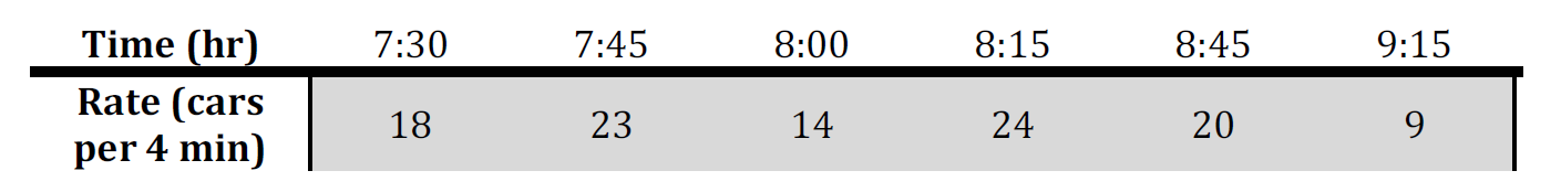
- Find the corresponding rate of cars through the intersection per minute
- By integrating the rate of cars per minute over the interval from 7:30 a.m. to 9:15 a.m., find the total number of cars that pass through the intersection. Use an appropriate integration method and justify its use.
Consider the following integral
$\int_{0}^3\!xe^{2x}\,\mathrm{d}x$
- Evaluate the integral analytically.
- Evaluate the integral using the Romberg’s method with a depth $k$ such that $\varepsilon_s=0.005$ .
- Evaluate the integral using the Gauss integration scheme with 1, 2, 3, and 4 integration point. Calculate the relative error in each case.
- Comment on the number of integration points required to achieve an acceptable accuracy.
Consider the following integral
$\mbox{erf}(a)=\frac{2}{\sqrt{\pi}}\int_{0}^{a}e^{-x^2}\,\mathrm{d}x$

with $a=1.5$
- Use the built-in numerical integration “NIntegrate” function to calculate an approximation to the true value of the integral. Consider this to be the true value.
- Evaluate the integral using the Gauss integration scheme with 1, 2, 3, and 4 integration point. Calculate the relative error in each case.
The amount of mass transported via a pipe over a period of time can be computed as:
$M=\int_{t_1}^{t_2}\!Q(t)c(t)\,\mathrm{d}t$

where $M$ is the mass in $mg$ , $t_1$ is the initial time in minutes, $t_2$ is the final time in minutes, $Q(t)$ is the flow rate in $m^3/min$ , and $c(t)$ is the concentration in $mg/m^3$ . The following functional representations define the temporal variations in flow and concentration:

$\begin{split} Q(t)&=9+5(\cos{(0.4t)} )^2\\ c(t)&=5e^{-0.5t}+2e^{0.15t} \end{split}$
- Determine the mass transported between $t_1=2$ and $t_2=8$ using the Gauss integration scheme with 1, 2, 3, and 4 integration points.
- Either using trial and error or using the upper bound of the error, find the number of intervals using the trapezoidal rule, and the Simpson’s 1/3 rule such that the absolute value of the error is equivalent to that produced by the Gauss integration scheme with 4 points.
- Find the level $k$ in the Romberg’s method that would produce an absolute value of the error similar to that produced by the Gauss integration scheme with 4 points.
Use the “Maximize” built-in function in Mathematica to create procedures whose inputs are $f$ , $h$ , $a$ , and $b$ which evaluate the upper bound of the error for the rectangle method, the trapezoidal rule, the Simpson’s 1/3 rule, and the Simpson’s 3/8 rule. Using different examples for each method, show that the actual error is indeed less than the upper bound of the error.
Modify the Romberg’s Method code so that the inputs are: $f$ , $a$ , $b$ , $k_{max}$ , and $\varepsilon_s$ . $k_{max}$ is the maximum number of columns in the produced Romberg table, but the code should stop when $\varepsilon_r\leq \varepsilon_s$ or when $k_{max}$ is reached. The code should be efficient such that the only terms that are calculated are those used in the estimate of the integral. (i.e., you should not calculate all the values up to $k_{max}$ ).

Open Educational Resources

Numerical Integration: Problems

Leave a Reply Cancel reply