
Ordinary Differential Equations: Solution Methods for BVPs
Solution Methods for BVPs
As mentioned above, BVP are ordinary differential equations whose boundary conditions are given at different values of the independent variable. Usually, these points are the extreme points of the region of interest, or the “boundaries” of the domain and hence the term: “boundary value problem”. Consider a BVP with  as the dependent variable and
  as the independent variable. The boundary conditions would be given in terms of or the derivatives of at different values of the independent variable . When the boundary conditions are given in terms of , then, this type of boundary conditions is termed Dirichlet boundary condition. Otherwise, when the boundary conditions are given in terms of the derivatives of , this type of boundary conditions is termed Neumann boundary condition. A BVP is usually an ODE that is at least of the second-order as equations of the first order require only one boundary condition which is usually an initial boundary condition. There are various methods to solve boundary value problems; among them are the following:
- Shooting method. In the shooting method the boundary value problem is solved as an initial value problem and the initial conditions are varied until the boundary conditions at the extreme ends are satisfied. For example, consider the BVP
![\[\frac{\mathrm{d}^2y}{\mathrm{d}x^2}=f(x)\]](https://engcourses-uofa.ca/wp-content/ql-cache/quicklatex.com-8f5ad3fb5a0c96d207854f76bd8d3c74_l3.png "Rendered by QuickLaTeX.com")
with the boundary conditions:![\[y(0)=y_0\qquad y(L)=y_L\]](https://engcourses-uofa.ca/wp-content/ql-cache/quicklatex.com-df1d332b5f8fc8d0ef52d17505db0f33_l3.png "Rendered by QuickLaTeX.com")
Then, the system can be converted into an initial value problem with the following boundary conditions:![\[y(0)=y_0\qquad y'(0)=s\]](https://engcourses-uofa.ca/wp-content/ql-cache/quicklatex.com-9866acd3d846e1629e5247b83ae9ebd4_l3.png "Rendered by QuickLaTeX.com")
After a solution is obtained, the value of is compared to
  and
and  is varied and the solution is repeated until
  .
. - Finite difference method. The finite difference method relies on approximating the BVP with difference equations by replacing the derivatives of the function with their finite difference approximations.
- Weak formulation methods. The weak formulation methods rely on converting the problem into a different “integral” form and finding the best solution that would satisfy the new form. Examples of such methods are the finite element analysis method or the weighted residuals methods.
The finite difference method is the only method that we will cover in these notes.
Finite Difference Method
Consider a BVP with the dependent variable and the independent variable with ![x\in[a,b]](https://engcourses-uofa.ca/wp-content/ql-cache/quicklatex.com-7bdc9e9b79b72dde0a30288760e0fe60_l3.png "Rendered by QuickLaTeX.com") . The finite difference method in a BVP relies on discretizing the domain
. The finite difference method in a BVP relies on discretizing the domain ![[a,b]](https://engcourses-uofa.ca/wp-content/ql-cache/quicklatex.com-1f90ba537767823131bb8d396cdc5a9c_l3.png "Rendered by QuickLaTeX.com") into
into  intervals with
  with a constant step size
  . The values of the dependent variable at the interval junctions are denoted by:
  . The finite difference method seeks to find a numerical solution to each
  by solving difference equations formed by replacing the derivatives in the BVP with a finite difference approximation scheme (usually the centred finite difference scheme). Dirichlet boundary conditions can be directly imposed on the known values of while Neumann boundary conditions can be imposed as additional difference equations using an appropriate finite difference scheme. The following examples show how the method can be implemented.
Example 1
In this example, we first derive the heat equation and then attempt to solve it using the finite difference method.
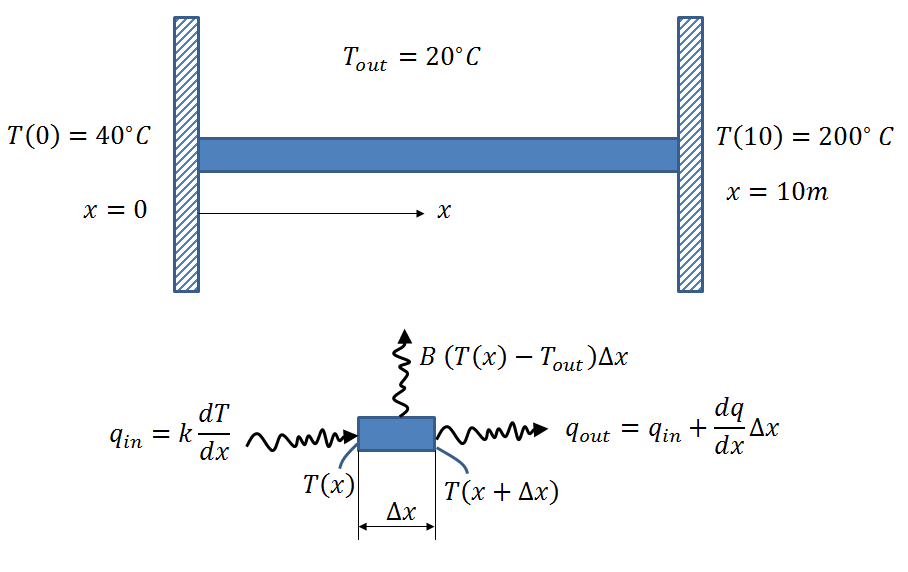
Heat Equation Derivation: The differential equation describing thermal energy within objects (Steady State Heat Equation) is one example of a BVP that can be solved using the finite difference method. In this example, the steady state heat equation is first derived for a one-dimensional rod of length 10m connecting two heat sources of constant temperature as shown in the figure such that the temperature of the rod at the end  is equal to
  C while the temperature at the other end
  is equal to
  C. The ambient temperature around the rod is equal to
  C. The steady state heat equation can be derived by balancing the amount of heat energy per unit time entering and exiting through a control length of the rod. The amount of heat energy transferred to the ambient environment per unit time and per unit length is equal to
![\[q_{\mbox{ambient}}=B(T(x)-T_{out})\]](https://engcourses-uofa.ca/wp-content/ql-cache/quicklatex.com-7c9a6343f64e8378625cbc2575acc3e5_l3.png "Rendered by QuickLaTeX.com")
With  units for this example. The amount of heat energy transferred through the rod per unit time is equal to:
![\[q_{in}=k\frac{\mathrm{d}T}{\mathrm{d}x}\]](https://engcourses-uofa.ca/wp-content/ql-cache/quicklatex.com-2d582faaac98974fab90ecc640887679_l3.png "Rendered by QuickLaTeX.com")
With  units in this example. The negative sign is essential as heat energy is transferred from areas of high temperature to areas of lower temperature. The steady state differential equation can be derived by equating the amount of energy entering to the amount of energy exiting per unit time considering a control length equal to
  as shown in the figure below:
![\[q_{in}=q_{\mbox{ambient}}+q_{out}= q_{\mbox{ambient}}+q_{in}+\frac{\mathrm{d}q}{\mathrm{d}x}\Delta x\]](https://engcourses-uofa.ca/wp-content/ql-cache/quicklatex.com-c33e66faf2fb45d83bb29f4e7116cece_l3.png "Rendered by QuickLaTeX.com")
Where a Taylor series with only two terms was used to approximate  . Therefore:
![\[\frac{\mathrm{d}^2T}{\mathrm{d}x^2}=\frac{1}{10}\left(T(x)-20 \right)\]](https://engcourses-uofa.ca/wp-content/ql-cache/quicklatex.com-b7a1ecac4a7533028e9e299152e4b9fb_l3.png "Rendered by QuickLaTeX.com")
The solution to this equation provides the temperature distribution (with  being the dependent variable) within the rod (with as the independent variable).
Statement of Problem: Consider the BVP developed above with the Dirichlet boundary conditions  and
and  .
.
- Find the exact solution of the differential equation.
- Use the finite difference method with
 intervals to find a numerical solution to the BVP.
Repeat the problem considering the two boundary conditions: the Dirichlet boundary condition and the Neumann boundary condition
![\[\frac{\mathrm{d}T}{\mathrm{d}x}\bigg|_{x=10}=-3\]](https://engcourses-uofa.ca/wp-content/ql-cache/quicklatex.com-ce38416a53dc32109095cb3b03846d41_l3.png "Rendered by QuickLaTeX.com")
Solution
Dirichlet Boundary Conditions
The exact solution can be directly obtained in Mathematica using the DSolve function. Note that an exact solution is not always available.
![\[T(x)= -4.80593 \sinh (0.316228 x)+20. \cosh (0.316228 x)+20.\]](https://engcourses-uofa.ca/wp-content/ql-cache/quicklatex.com-5ff6f429b1884f96afefa0f7a669b701_l3.png "Rendered by QuickLaTeX.com")
The numerical solution is obtained by first discretizing the domain into intervals with  and
and  . The values of at these points are denoted by
  . The boundary conditions are given as Dirichlet type with
  and
and  . The remaining 3 unknowns can be obtained by utilizing the basic formulas of the centred finite difference scheme to replace the derivatives in the differential equation. These can be utilized to write 4 equations of the form:
![\[\frac{T_{i+1}-2T_i+T_{i-1}}{h^2} =\frac{1}{10}\left(T_i-20\right)\]](https://engcourses-uofa.ca/wp-content/ql-cache/quicklatex.com-ecdc68bcdbbe207e3a7ad64739348f2a_l3.png "Rendered by QuickLaTeX.com")
This results in the following three equations (after the substitution and ):
![\[\begin{split}\frac{T_2-2T_1+40}{6.25} &=\frac{1}{10}\left(T_1-20\right)\\\frac{T_3-2T_2+T_1}{6.25} &=\frac{1}{10}\left(T_2-20\right)\\\frac{200-2T_3+T_2}{6.25} &=\frac{1}{10}\left(T_3-20\right)\end{split}\]](https://engcourses-uofa.ca/wp-content/ql-cache/quicklatex.com-220172131f722d26c8d4199dd9be13e7_l3.png "Rendered by QuickLaTeX.com")
Rearranging yields the following linear system of equations:
![\[\left(\begin{matrix}-0.42&0.16&0\\0.16&-0.42&0.16\\0&0.16&-0.42 \end{matrix}\right)\left(\begin{array}{c}T_1\\T_2\\T_3\end{array}\right)=\left(\begin{array}{c}-8.4\\-2\\-34\end{array}\right)\]](https://engcourses-uofa.ca/wp-content/ql-cache/quicklatex.com-ed107d93a6390ff15c1390a168a7a815_l3.png "Rendered by QuickLaTeX.com")
Solving the above system yields:
![\[\left(\begin{array}{c}T_1\\T_2\\T_3\end{array}\right)=\left(\begin{array}{c}43.1979\\60.8946\\104.15\end{array}\right)\]](https://engcourses-uofa.ca/wp-content/ql-cache/quicklatex.com-5f5b9342652a4a45d63ce48eb8b46eba_l3.png "Rendered by QuickLaTeX.com")
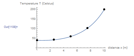
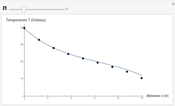
Combined with and , a list plot can be drawn to show the obtained numerical solution. The following figure shows the exact solution (blue curve) with the numerical solution (black dots). The figure shows that the numerical solution is almost identical to the exact solution.
ClearAll["Global`*"]
hp = 1/10;
n = 4;
L = 10 - 0;
h = L/n;
Ts = Table[Symbol["T" <> ToString[i]], {i, 0, n}]
T0 = 40;
Ts[[n + 1]] = 200;
Ts // MatrixForm
Equations =   Table[(Ts[[i + 1]] - 2 Ts[[i]] + Ts[[i - 1]])/h^2 ==     hp*(Ts[[i]] - 20), {i, 2, n}];
Equations // MatrixForm
Equations = Expand[Equations];
Equations // MatrixForm
N[Equations] // MatrixForm

unknowns = Table[Symbol["T" <> ToString[i]], {i, 1, n - 1}]
a = Solve[Equations, unknowns]
Ts = Ts /. a[[1]]
SolList = Table[{0 + (i)*h, Ts[[i + 1]]}, {i, 0, n}];
SolList // MatrixForm

a = DSolve[{T''[x] == hp*(T[x] - 20), T[0] == 40, T[10] == 200}, T, x]
T = T[x] /. a[[1]];
FullSimplify[N[T]]
Plot[T, {x, 0, 10},  AxesLabel -> {"distance x (m)", "Temperature T (Celsius)"},  AxesOrigin -> {0, 0}, Epilog -> {PointSize[Large], Point[SolList]}]
# UPGRADE: need Sympy 1.2 or later, upgrade by running: "!pip install sympy --upgrade" in a code cell
# !pip install sympy --upgrade
import numpy as np
import sympy as sp
import matplotlib.pyplot as plt
sp.init_printing(use_latex=True)

hp = 1/10
n = int(4)
L = 10
h = L/n
x = sp.symbols('x')
T = sp.Function('T')
Ts = [T(i) for i in range(n+1)]
Ts[n] = 200
Ts[0] = 40
print(Ts)
Equations = [sp.Eq((Ts[i + 1] - 2*Ts[i] + Ts[i - 1])/h**2, hp*(Ts[i] - 20)) for i in range(1,n)]
display(sp.Matrix(Equations))
Equations = [sp.factor(equation) for equation in Equations]
display(sp.Matrix(Equations))

unknowns = [T(i) for i in range(1, n)]
display(unknowns)
sol = list(sp.linsolve(Equations, unknowns))
display(sol)
for i in range(1, n):
  Ts[i] = sol[0][i-1]
display(Ts)
SolList = [[i*h, Ts[i]] for i in range(n+1)]
display(sp.Matrix(SolList))

sol = sp.dsolve(T(x).diff(x,2) - hp*(T(x) - 20), ics={T(0): 40, T(10): 200})
display(sol)

x_val = np.arange(0,10,0.01)
plt.plot(x_val, [sol.subs(x, i).rhs for i in x_val])
plt.scatter([point[0] for point in SolList],
            [point[1] for point in SolList],c='k')
plt.xlabel("Distance x (m)"); plt.ylabel("Temperature T (Celsius)")
plt.grid(); plt.show()
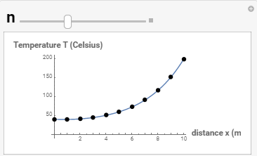
In the following tool, vary the number of intervals to show the effect on the numerical solution:
Dirichlet and Neumann Boundary Conditions
The exact solution can be directly obtained in Mathematica using the DSolve function. Note that an exact solution is not always available.
![\[T(x)= -20.7302 \sinh (0.316228 x)+20. \cosh (0.316228 x)+20.\]](https://engcourses-uofa.ca/wp-content/ql-cache/quicklatex.com-7a24a3cb5cff2549effbe8cd18037da7_l3.png "Rendered by QuickLaTeX.com")
The numerical solution is obtained by first discretizing the domain into intervals with and . The values of at these points are denoted by . The Dirichlet boundary condition can be used to set . The remaining 4 unknowns can be obtained using four equations. Three equations are composed by utilizing the basic formulas of the centred finite difference scheme to replace the derivatives in the differential equation at the three intermediate points. The fourth equation is composed by utilizing the backward finite difference scheme at  and equate it to the Neumann boundary condition. The three difference equations at the intermediate points have the form:
This results in the following three equations (after the substitution ):
![\[\begin{split}\frac{T_2-2T_1+40}{6.25} &=\frac{1}{10}\left(T_1-20\right)\\\frac{T_3-2T_2+T_1}{6.25} &=\frac{1}{10}\left(T_2-20\right)\\\frac{T_4-2T_3+T_2}{6.25} &=\frac{1}{10}\left(T_3-20\right)\end{split}\]](https://engcourses-uofa.ca/wp-content/ql-cache/quicklatex.com-4f47ef3f5635ac469f35dbcaf674bd31_l3.png "Rendered by QuickLaTeX.com")
The fourth equation can be obtained using the backward finite difference at point :
![\[\frac{T_4-T_3}{2.5}=-3\]](https://engcourses-uofa.ca/wp-content/ql-cache/quicklatex.com-a8f89b1c75ff21baf3a4cb3b5baedacc_l3.png "Rendered by QuickLaTeX.com")
Combining the four equations and rearranging yields the following linear system of equations:
![\[\left(\begin{matrix}-0.42&0.16&0&0\\0.16&-0.42&0.16&0\\0&0.16&-0.42&0.16\\0&0&-0.4&0.4 \end{matrix}\right)\left(\begin{array}{c}T_1\\T_2\\T_3\\T_4\end{array}\right)=\left(\begin{array}{c}-8.4\\-2\\-2\\-3\end{array}\right)\]](https://engcourses-uofa.ca/wp-content/ql-cache/quicklatex.com-ab757785835f45dd44d1278549089258_l3.png "Rendered by QuickLaTeX.com")
Solving the above system yields:
![\[\left(\begin{array}{c}T_1\\T_2\\T_3\\T_4\end{array}\right)=\left(\begin{array}{c}28.3216\\21.8443\\16.5195\\9.01954\end{array}\right)\]](https://engcourses-uofa.ca/wp-content/ql-cache/quicklatex.com-e2fa126e7b8781b9cb2436fdf280b1c3_l3.png "Rendered by QuickLaTeX.com")
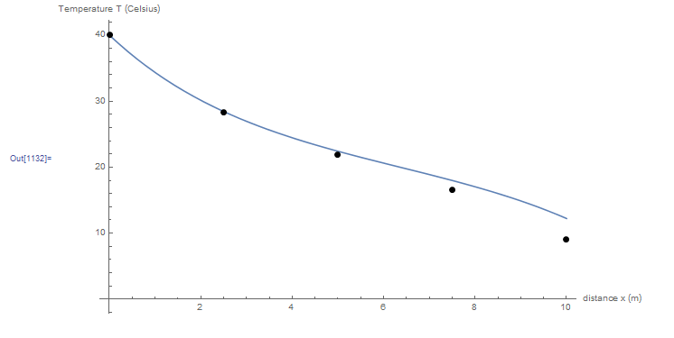
Combined with , a list plot can be drawn to show the obtained numerical solution. The following figure shows the exact solution (blue curve) with the numerical solution (black dots). The figure shows that the numerical solution of the same differential equation with Neumann boundary conditions provides less accurate results than the solution when Dirichlet boundary conditions were used.
ClearAll["Global`*"]
hp = 1/10;
n = 4;
L = 10 - 0;
h = L/n;
Ts = Table[Symbol["T" <> ToString[i]], {i, 0, n}]
T0 = 40;
Ts // MatrixForm
Equations =   Table[(Ts[[i + 1]] - 2 Ts[[i]] + Ts[[i - 1]])/h^2 ==     hp*(Ts[[i]] - 20), {i, 2, n}];
NeumannEquation = ((Ts[[n + 1]] - Ts[[n]])/h == -3);
Equations = Append[Equations, NeumannEquation];
Equations // MatrixForm
Equations = Expand[Equations];
Equations // MatrixForm
N[Equations] // MatrixForm

unknowns = Table[Symbol["T" <> ToString[i]], {i, 1, n}]
a = Solve[Equations, unknowns];
Ts = N[Ts /. a[[1]]]
SolList = Table[{0 + (i)*h, Ts[[i + 1]]}, {i, 0, n}];
SolList // MatrixForm

a = DSolve[{T''[x] == hp*(T[x] - 20), T[0] == 40, T'[10] == -3}, T, x]
T = T[x] /. a[[1]];
FullSimplify[N[T]]
Plot[T, {x, 0, 10},  AxesLabel -> {"distance x (m)", "Temperature T (Celsius)"},  AxesOrigin -> {0, 0}, Epilog -> {PointSize[Large], Point[SolList]}]
# UPGRADE: need Sympy 1.2 or later, upgrade by running: "!pip install sympy --upgrade" in a code cell
# !pip install sympy --upgrade
import numpy as np
import sympy as sp
import matplotlib.pyplot as plt
sp.init_printing(use_latex=True)

hp = 1/10
n = int(4)
L = 10
h = L/n
x = sp.symbols('x')
T = sp.Function('T')
Ts = [T(i) for i in range(n+1)]
Ts[0] = 40
display(Ts)
Equations = [sp.Eq((Ts[i + 1] - 2*Ts[i] + Ts[i - 1])/h**2, hp*(Ts[i] - 20)) for i in range(1,n)]
NeumannEquation = sp.Eq((Ts[n] - Ts[n - 1])/h, -3)
Equations.append(NeumannEquation)
display(sp.Matrix(Equations))
Equations = [sp.factor(equation) for equation in Equations]
display(sp.Matrix(Equations))

unknowns = [T(i) for i in range(1, n+1)]
display(unknowns)
sol = list(sp.linsolve(Equations, unknowns))
display(sol)
for i in range(1, n+1):
  Ts[i] = sol[0][i-1]
display(Ts)
SolList = [[i*h, Ts[i]] for i in range(n+1)]
display(sp.Matrix(SolList))

sol = sp.dsolve(T(x).diff(x,2) - hp*(T(x) - 20), ics={T(0): 40, T(x).diff(x).subs(x,10): -3})
display(sol)

x_val = np.arange(0,10,0.01)
plt.plot(x_val, [sol.subs(x, i).rhs for i in x_val])
plt.scatter([point[0] for point in SolList],
            [point[1] for point in SolList],c='k')
plt.xlabel("Distance x (m)"); plt.ylabel("Temperature T (Celsius)")
plt.grid(); plt.show()
The numerical solution approaches the exact solution as the number of intervals is increased. Vary in the following tool and observe how it affects the numerical solution.
Example 2
Consider the following second-order BVP:
![\[u''(x)+u'(x)+u(x)=1\]](https://engcourses-uofa.ca/wp-content/ql-cache/quicklatex.com-2a04108abbd2ad2886a00464155d140b_l3.png "Rendered by QuickLaTeX.com")
with the boundary conditions:
![\[u(0)=1.5\qquad u(3)=2.5\]](https://engcourses-uofa.ca/wp-content/ql-cache/quicklatex.com-61fb084d33e69774ee39cbc2f225cb10_l3.png "Rendered by QuickLaTeX.com")
Use the finite difference method to find a numerical solution to the above equation by dividing the domain ![x\in[0,3]](https://engcourses-uofa.ca/wp-content/ql-cache/quicklatex.com-f38aec68cb3f3acfd3f49bd8a175b5ff_l3.png "Rendered by QuickLaTeX.com") into
into  intervals. Compare with the exact solution.
Solution
The exact solution can be directly obtained in Mathematica using the DSolve function. Note that an exact solution is not always available.
![\[u=\frac{1}{2} e^{-\frac{x}{2}} \left(2 e^{\frac{x}{2}}+\cos \left(\frac{\sqrt{3} x}{2}\right)-\left(\cos \left(\frac{3 \sqrt{3}}{2}\right)-3 e^{3/2}\right) \csc \left(\frac{3 \sqrt{3}}{2}\right) \sin \left(\frac{\sqrt{3} x}{2}\right)\right)\]](https://engcourses-uofa.ca/wp-content/ql-cache/quicklatex.com-06258b9fff49121a86bd50a49f597205_l3.png "Rendered by QuickLaTeX.com")
The numerical solution is obtained by first discretizing the domain into intervals with  and
and  . The values of
  at these points are denoted by
  . The boundary conditions are given as Dirichlet type with
  and
and  . The remaining 4 unknowns can be obtained by utilizing the basic formulas of the centred finite difference scheme to replace the derivatives in the differential equation. These can be utilized to write 4 equations of the form:
![\[\frac{u_{i+1}-2u_i+u_{i-1}}{h^2}+\frac{u_{i+1}-u_{i-1}}{2h}+u_i=1\]](https://engcourses-uofa.ca/wp-content/ql-cache/quicklatex.com-b8dd89e3c908f3fb12ef5f0500abc9b3_l3.png "Rendered by QuickLaTeX.com")
This results in the following four equations (after the substitution and ):
![\[\begin{split}\frac{u_{2}-2u_1+1.5}{0.36}+\frac{u_{2}-1.5}{1.2}+u_1&=1\\\frac{u_{3}-2u_2+u_1}{0.36}+\frac{u_{3}-u_1}{1.2}+u_2&=1\\\frac{u_{4}-2u_3+u_2}{0.36}+\frac{u_{4}-u_2}{1.2}+u_3&=1\\\frac{2.5-2u_4+u_3}{0.36}+\frac{2.5-u_3}{1.2}+u_4&=1\end{split}\]](https://engcourses-uofa.ca/wp-content/ql-cache/quicklatex.com-8fe649c16c2e5c7b6409f3f6b144811b_l3.png "Rendered by QuickLaTeX.com")
Rearranging yields the following linear system of equations:
![\[\left(\begin{matrix}-4.556&3.611&0&0\\1.944&-4.556&3.611&0\\0&1.944&-4.556&3.611\\0&0&1.944&-4.556\end{matrix}\right)\left(\begin{array}{c}u_1\\u_2\\u_3\\u_4\end{array}\right)=\left(\begin{array}{c}-1.91667\\1\\1\\-8.02778\end{array}\right)\]](https://engcourses-uofa.ca/wp-content/ql-cache/quicklatex.com-18934aecb8849193879a12102a2c1781_l3.png "Rendered by QuickLaTeX.com")
Solving the above system yields:
![\[\left(\begin{array}{c}u_1\\u_2\\u_3\\u_4\end{array}\right)=\left(\begin{array}{c}7.649\\9.1183\\7.6615\\5.0323\end{array}\right)\]](https://engcourses-uofa.ca/wp-content/ql-cache/quicklatex.com-deba8801f47899c3d321d1ac368b4a87_l3.png "Rendered by QuickLaTeX.com")
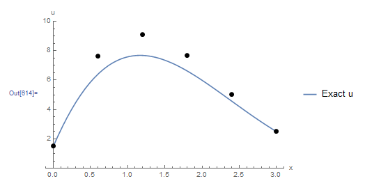
Combined with and , a list plot can be drawn to show the obtained numerical solution. The following figure shows the exact solution (blue curve) with the numerical solution (black dots). The maximum error in the numerical solution is obtained at  . At this location, the exact solution is given by
  while the numerical solution is given by
  with a relative error of -19%:
![\[E_r=\frac{7.68-9.12}{7.68}=-0.19\]](https://engcourses-uofa.ca/wp-content/ql-cache/quicklatex.com-0d5846ec3921d646ec904dafcdca9b3c_l3.png "Rendered by QuickLaTeX.com")
 View Mathematica Code
ClearAll["Global`*"]
n = 5;
L = 3 - 0;
h = L/n;
us = Table[Symbol["u" <> ToString[i]], {i, 0, n}]
u0 = 1.5;
us[[n + 1]] = 2.5;
us // MatrixForm
Equations = Table[(us[[i + 1]] - 2 us[[i]] + us[[i - 1]])/h^2 + (us[[i + 1]] - us[[i - 1]])/2/h + us[[i]] == 1, {i, 2, n}];
Equations // MatrixForm
Equations = Expand[Equations];
Equations // MatrixForm
N[Equations] // MatrixForm

unknowns = Table[Symbol["u" <> ToString[i]], {i, 1, n - 1}]
a = Solve[Equations, unknowns]
us = us /. a[[1]]
SolList = Table[{0 + (i)*h, us[[i + 1]]}, {i, 0, n}];
SolList // MatrixForm;

Clear[u]
(*Exact Solution*)
b = DSolve[{u''[x] + u'[x] + u[x] == 1, u[0] == 15/10, u[3] == 25/10},   u, x]
u = FullSimplify[u[x] /. b[[1]], Reals]
Plot[u, {x, 0, 3}, PlotLegends -> {"Exact u"},  AxesLabel -> {"x", "u"},  Epilog -> {PointSize[Large], Point[SolList]},  PlotRange -> {{-0.1, 3.1}, {0, 10}}]
Print["u at x=1.2 is ", uexact = u /. x -> 1.2]
Print["u_2 is ", u2 = u2 /. a[[1]]]
Print["Relative Error is ", (uexact - u2)/uexact]
# UPGRADE: need Sympy 1.2 or later, upgrade by running: "!pip install sympy --upgrade" in a code cell
# !pip install sympy --upgrade
import numpy as np
import sympy as sp
import matplotlib.pyplot as plt
sp.init_printing(use_latex=True)

n = int(5)
L = 3
h = L/n
x = sp.symbols('x')
u = sp.Function('u')
us = [u(i) for i in range(n+1)]
us[0] = 1.5
us[n] = 2.5
display(us)
Equations = [sp.Eq((us[i + 1] - 2*us[i] + us[i - 1])/h**2 + (us[i + 1] - us[i - 1])/2/h + us[i], 1) for i in range(1,n)]
display(sp.Matrix(Equations))

unknowns = [u(i) for i in range(1, n)]
display(unknowns)
sol = list(sp.linsolve(Equations, unknowns))
display(sol)
for i in range(1, n):
  us[i] = sol[0][i-1]
display(us)
SolList = [[i*h, us[i]] for i in range(n+1)]
display(sp.Matrix(SolList))

# Exact Solution
u = sp.dsolve(u(x).diff(x,2) + u(x).diff(x) + u(x) - 1, ics={u(0): 15/10, u(3): 25/10})
display(u)

uexact = sp.N(u.subs(x, 1.2).rhs)
print("u at x = 1.2 is", uexact)
print("u_2 is", us[2])
print("Relative Error is", (uexact - us[2])/uexact)

x_val = np.arange(0,3,0.01)
plt.plot(x_val, [u.subs(x, i).rhs for i in x_val], label="Exact u")
plt.scatter([point[0] for point in SolList],
            [point[1] for point in SolList],c='k')
plt.xlabel("x"); plt.ylabel("u")
plt.legend(); plt.grid(); plt.show()
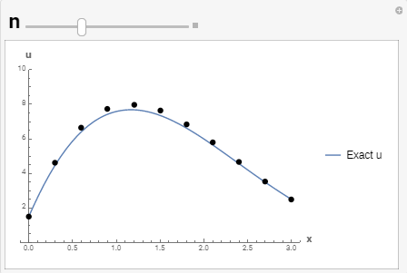
In a BVP, the accuracy of the solution depends on the accuracy of the finite difference scheme used. As shown in the following tool, by decreasing the value of  , the numerical solution gets closer to the exact solution.
Example 3
The differential equation describing the displacement of a hanging chain as a function of the weight per unit length  of the chain and the desired horizontal tension in the chain
  is given by:
![\[\frac{\mathrm{d}^2y}{\mathrm{d}x^2}=\frac{w}{T_0}\sqrt{1+\left(\frac{\mathrm{d}y}{\mathrm{d}x}\right)^2}\]](https://engcourses-uofa.ca/wp-content/ql-cache/quicklatex.com-e856638222e723d18664233e9a98a74a_l3.png "Rendered by QuickLaTeX.com")
Where is the dependent variable being the chain curve and is the independent variable being the horizontal distance. The solution to this equation, namely the function  is called the catenary or the curve that describes the hanging chain. See this page for a detailed derivation and some of the properties of the curve.
If the boundary conditions are given by  and
and  and if
  and
and  units, then use the finite difference method to find a numerical solution by dividing the domain
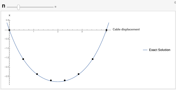
 ![x\in[0,4]](https://engcourses-uofa.ca/wp-content/ql-cache/quicklatex.com-44f948b65f3f419f062bde88157f55b2_l3.png "Rendered by QuickLaTeX.com") into intervals. Compare with the exact solution.
into intervals. Compare with the exact solution.
Solution
Notice that this equation is a nonlinear second-order differential equation. Its exact solution describing the catenary of the chain can be obtained using the built-in Integrate function in Mathematica and has the form:
![\[y= \cosh (2-x)-\cosh (2)=\frac{1}{2}\left(e^{2-x}+e^{x-2}-e^{2}-e^{-2}\right)\]](https://engcourses-uofa.ca/wp-content/ql-cache/quicklatex.com-cb3dfc44df0a6780499be4b07138d9bc_l3.png "Rendered by QuickLaTeX.com")
The numerical solution is obtained by first discretizing the domain into intervals with  and
and  . The values of at these points are denoted by
  . The boundary conditions are given as Dirichlet type with
  and
and  . The remaining 4 unknowns can be obtained by utilizing the basic formulas of the centred finite difference scheme to replace the derivatives in the differential equation. These can be utilized to write 4 nonlinear equations of the form:
![\[\frac{y_{i+1}-2y_i+y_{i-1}}{h^2}=\sqrt{1+\left(\frac{y_{i+1}-y_{i-1}}{2h}\right)^2}\]](https://engcourses-uofa.ca/wp-content/ql-cache/quicklatex.com-0c3602bf0dced331ea4e031f1ddbfefd_l3.png "Rendered by QuickLaTeX.com")
This results in the following four nonlinear equations (after the substitution and ):
![\[\begin{split}\frac{y_2-2y_1+0}{0.64}&=\sqrt{1+\left(\frac{y_2-0}{1.6}\right)^2}\\\frac{y_3-2y_2+y_1}{0.64}&=\sqrt{1+\left(\frac{y_3-y_1}{1.6}\right)^2}\\\frac{y_4-2y_3+y_2}{0.64}&=\sqrt{1+\left(\frac{y_4-y_2}{1.6}\right)^2}\\\frac{0-2y_4+y_3}{0.64}&=\sqrt{1+\left(\frac{0-y_3}{1.6}\right)^2}\end{split}\]](https://engcourses-uofa.ca/wp-content/ql-cache/quicklatex.com-dc12fdf310429bf182c94b17f9a6c249_l3.png "Rendered by QuickLaTeX.com")
Notice that the resulting equations are nonlinear because the differential equation itself was nonlinear. The above system can be solved using the Newton-Raphson method with initial guesses of  for all of the unknowns which yields the following solution:
![\[\left(\begin{array}{c}y_1\\y_2\\y_3\\y_4\end{array}\right)=\left(\begin{array}{c}-1.92863\\-2.62693\\-2.62693\\-1.92863\end{array}\right)\]](https://engcourses-uofa.ca/wp-content/ql-cache/quicklatex.com-4236f0d8501521ddc4802fd11938653c_l3.png "Rendered by QuickLaTeX.com")
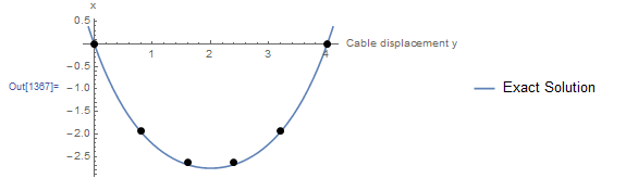
Combined with and , a list plot can be drawn to show the obtained numerical solution. The following figure shows the exact solution (blue curve) with the numerical solution (black dots). The two solutions are very close to each other.
 View Mathematica Code
ClearAll["Global`*"]
w = 1.;
T = 1;
a = DSolve[{y''[x] == w/T*Sqrt[1 + (y'[x])^2], y[0] == 0, y[4] == 0},y, x]
y = FullSimplify[y[x] /. a[[1]]]
Plot[y, {x, 0, 4}]
L = 4 - 0
n = 5;
h = L/n;
ys = Table[Symbol["y" <> ToString[i]], {i, 0, n}];
y0 = 0;
ys[[n + 1]] = 0;
ys // MatrixForm
Equations =   Table[(ys[[i + 1]] - 2 ys[[i]] + ys[[i - 1]])/h^2 ==     w/T*Sqrt[1 + ((ys[[i + 1]] - ys[[i - 1]])/2/h)^2], {i, 2, n}];
Equations // MatrixForm
unknowns = Table[Symbol["y" <> ToString[i]], {i, 1, n - 1}];
Initvalues = Table[{unknowns[[i]], -0.1}, {i, 1, n - 1}];
a = FindRoot[Equations, Initvalues]
ys = ys /. a
SolList = Table[{0 + (i)*h, ys[[i + 1]]}, {i, 0, n}];
Plot[y, {x, -0.1, 4.1}, AxesLabel -> {"Cable displacement y", "x"}, PlotLegends -> {"Exact Solution"},  Epilog -> {PointSize[Large], Point[SolList]}]
# UPGRADE: need Sympy 1.2 or later, upgrade by running: "!pip install sympy --upgrade" in a code cell
# !pip install sympy --upgrade
import numpy as np
import sympy as sp
import matplotlib.pyplot as plt
from scipy.optimize import root
sp.init_printing(use_latex=True)

w = 1
T = 1
L = 4
n = int(5)
h = L/n

x = sp.symbols('x')
y = sp.Function('y')
dsol = sp.dsolve(y(x).diff(x,2) - w/T*sp.sqrt(1 + (y(x).diff(x))**2), hint="nth_order_reducible")
display("dsolve:",dsol)
constants = sp.solve([dsol.rhs.subs(x,0), dsol.rhs.subs(x,4)])
display("constants:",constants)
sol = dsol.subs(constants[0])
display("sol:",sol)
x_val = np.arange(0,4,0.01)
plt.plot(x_val, [sol.subs(x, i).rhs for i in x_val])
plt.grid(); plt.show()

ys = [y(i) for i in range(n + 1)]
ys[0] = 0
ys[n] = 0
display("ys:",ys)
Equations = [sp.simplify((ys[i + 1] - 2*ys[i] + ys[i - 1])/h**2 - w/T*sp.sqrt(1 + ((ys[i + 1] - ys[i - 1])/2/h)**2)) for i in range(1,n)]
print(Equations)
display("Equations:",sp.Matrix(Equations))

# Convert Sympy equations to a Python function using lambdify
equations = sp.lambdify(((y(1), y(2), y(3), y(4)),), Equations)
# Solve system of equations using Scipy's root
rootSol = root(equations, [0,0,0,0])
print("[y1 y2 y3 y4] = ",rootSol.x)
SolList = [0] + list(rootSol.x) + [0]
print("SolList:",SolList)

x_val = np.arange(-0.1,4.1,0.01)
plt.plot(x_val, [sol.subs(x, i).rhs for i in x_val], label="Exact Solution")
plt.scatter([i*h for i in range(n+1)], SolList, c='k')
plt.xlabel("Cable displacement y"); plt.ylabel("x")
plt.legend(); plt.grid(); plt.show()
As shown in the following tool, by decreasing the value of , the numerical solution gets closer to the exact solution.
Example 4
Consider the following BVP
![\[7\frac{\mathrm{d}^2y}{\mathrm{d}x^2}-2\frac{\mathrm{d}y}{\mathrm{d}x}-y+x=0\]](https://engcourses-uofa.ca/wp-content/ql-cache/quicklatex.com-cdf616b2b6dc42240c5d1718f69d8b85_l3.png "Rendered by QuickLaTeX.com")
With the boundary conditions  and
and  . Assuming
  , use the finite difference method to find a numerical solution to the given BVP. Compare with the exact solution.
Solution
The exact solution can be directly obtained in Mathematica using the DSolve function.
![\[y= x+7.00018 e^{-0.261204 x}-0.000178305 e^{0.546918 x}-2.\]](https://engcourses-uofa.ca/wp-content/ql-cache/quicklatex.com-b277cfb2d5cbd1e16d2358dad62717bb_l3.png "Rendered by QuickLaTeX.com")
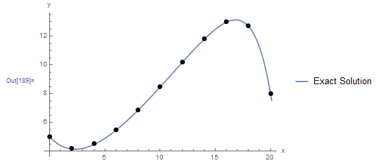
The numerical solution is obtained by first discretizing the domain into  intervals with
  and
and  ,
,  . The values of at these points are denoted by
  . The boundary conditions are given as Dirichlet type with
  and
and  . The remaining 9 unknowns can be obtained by utilizing the basic formulas of the centred finite difference scheme to replace the derivatives in the differential equation. These can be utilized to write 9 equations of the form:
![\[7\left(\frac{y_{i+1}-2y_i+y_{i-1}}{h^2}\right)-2\left(\frac{y_{i+1}-y_{i-1}}{2h}\right)-y_i+x_i=0\]](https://engcourses-uofa.ca/wp-content/ql-cache/quicklatex.com-583932c33583f4caacd39e813a32befc_l3.png "Rendered by QuickLaTeX.com")
This results in the following nine equations (after the substitution and ):
![\[\begin{split}7\left(\frac{y_2-2y_1+5}{4}\right)-\frac{y_2-5}{2}-y_1+x_1&=0\\7\left(\frac{y_3-2y_2+y_1}{4}\right)-\frac{y_3-y_1}{2}-y_2+x_2&=0\\7\left(\frac{y_4-2y_3+y_2}{4}\right)-\frac{y_4-y_2}{2}-y_3+x_3&=0\\7\left(\frac{y_5-2y_4+y_3}{4}\right)-\frac{y_5-y_3}{2}-y_4+x_4&=0\\7\left(\frac{y_6-2y_5+y_4}{4}\right)-\frac{y_6-y_4}{2}-y_5+x_5&=0\\7\left(\frac{y_7-2y_6+y_5}{4}\right)-\frac{y_7-y_5}{2}-y_6+x_6&=0\\7\left(\frac{y_8-2y_7+y_6}{4}\right)-\frac{y_8-y_6}{2}-y_7+x_7&=0\\7\left(\frac{y_9-2y_8+y_7}{4}\right)-\frac{y_9-y_7}{2}-y_8+x_8&=0\\7\left(\frac{8-2y_9+y_8}{4}\right)-\frac{8-y_8}{2}-y_9+x_9&=0\end{split}\]](https://engcourses-uofa.ca/wp-content/ql-cache/quicklatex.com-6f1b344b88eb21d49b4de14c028ab9ec_l3.png "Rendered by QuickLaTeX.com")
Rearranging yields the following linear system of equations:
![\[\left(\begin{matrix}-4.5&1.25&0&0&0&0&0&0&0\\2.25&-4.5&1.25&0&0&0&0&0&0\\0&2.25&-4.5&1.25&0&0&0&0&0\\0&0&2.25&-4.5&1.25&0&0&0&0\\0&0&0&2.25&-4.5&1.25&0&0&0\\0&0&0&0&2.25&-4.5&1.25&0&0\\0&0&0&0&0&2.25&-4.5&1.25&0\\0&0&0&0&0&0&2.25&-4.5&1.25\\0&0&0&0&0&0&0&2.25&-4.5\end{matrix}\right)\left(\begin{array}{c}y_1\\y_2\\y_3\\y_4\\y_5\\y_6\\y_7\\y_8\\y_9\end{array}\right)=\left(\begin{array}{c}-13.25\\-4\\-6\\-8\\-10\\-12\\-14\\-16\\-28\end{array}\right)\]](https://engcourses-uofa.ca/wp-content/ql-cache/quicklatex.com-e6d860f7c4c6a483184c6d1504dbd382_l3.png "Rendered by QuickLaTeX.com")
Solving the above system yields:
![\[\left(\begin{array}{c}y_1\\y_2\\y_3\\y_4\\y_5\\y_6\\y_7\\y_8\\y_9\end{array}\right)=\left(\begin{array}{c}4.19959\\4.51853\\5.50744\\6.89345\\8.50301\\10.2026\\11.824\\13.0018\\12.7231\end{array}\right)\]](https://engcourses-uofa.ca/wp-content/ql-cache/quicklatex.com-e3b70f297bb8588a1e814a92f45334db_l3.png "Rendered by QuickLaTeX.com")
Combined with and , a list plot can be drawn to show the obtained numerical solution. The following figure shows the exact solution (blue curve) with the numerical solution (black dots). The numerical solution provides a very good approximation to the the exact solution!
ClearAll["Global`*"]
a = DSolve[{7 y''[x] - 2 y'[x] - y[x] + x == 0, y[0] == 5, y[20] == 8}, y, x]
y = FullSimplify[y[x] /. a[[1]]]
y = FullSimplify[N[y]]
Plot[y, {x, 0, 20}]
L = 20 - 0
n = 10;
h = L/n;
ys = Table[Symbol["y" <> ToString[i]], {i, 0, n}];
y0 = 5;
ys[[n + 1]] = 8;
ys // MatrixForm
Equations =   Table[7 (ys[[i + 1]] - 2 ys[[i]] + ys[[i - 1]])/h^2 -      2 (ys[[i + 1]] - ys[[i - 1]])/2/h - ys[[i]] + 0 + (i - 1)*h ==     0, {i, 2, n}];
Equations // MatrixForm
Expand[N[Equations]] // MatrixForm
unknowns = Table[Symbol["y" <> ToString[i]], {i, 1, n - 1}];
a = Solve[Equations, unknowns];
ys = N[ys /. a[[1]]]
SolList = Table[{0 + (i)*h, ys[[i + 1]]}, {i, 0, n}];
Plot[y, {x, -0.1, 20.1}, AxesLabel -> {"x", "y"},  PlotLegends -> {"Exact Solution"},  Epilog -> {PointSize[Large], Point[SolList]}]
import numpy as np
import sympy as sp
import matplotlib.pyplot as plt
sp.init_printing(use_latex=True)

x = sp.symbols('x')
y = sp.Function('y')
a = sp.dsolve(7*y(x).diff(x,2) - 2*y(x).diff(x) - y(x) + x, ics={y(0): 5, y(20): 8})
display(a)
a = sp.simplify(a)
display(a)
x_val = np.arange(0,20.1,0.1)
plt.plot(x_val, [a.subs(x, i).rhs for i in x_val])
plt.grid(); plt.show()

L = 20
n = 10
h = L/n
ys = [y(i) for i in range(n+1)]
ys[0] = 5
ys[n] = 8
display(ys)
Equations = [sp.Eq(7*(ys[i + 1] - 2*ys[i] + ys[i - 1])/h**2 - 2*(ys[i + 1] - ys[i - 1])/2/h - ys[i] + i*h, 0) for i in range(1,n)]
display(sp.Matrix(Equations))
unknowns = [y(i) for i in range(1,n)]
display(unknowns)
sol = list(sp.linsolve(Equations, unknowns))
display(sol)
for i in range(1, n):
  ys[i] = sol[0][i-1]
display(ys)
SolList = [[i*h, ys[i]] for i in range(n+1)]
display(sp.Matrix(SolList))

plt.plot(x_val, [a.subs(x, i).rhs for i in x_val], label="Exact Solution")
plt.scatter([point[0] for point in SolList],
            [point[1] for point in SolList],c='k')
plt.xlabel("x"); plt.ylabel("y")
plt.legend(); plt.grid(); plt.show()
hello sirs, thank you for this guidance but what happen when an equation has two dependent variables and one independent variable then how can we solve them by finite difference method can you provide some knowledge for this or i suggest that give me a solution pattern of this type of question
thanks