Introduction to Numerical Analysis: Numerical Differentiation

Introduction

Let be a smooth (differentiable) function, then the derivative of at is defined as the limit:

When is an explicit function of , one can often find an expression for the derivative of . For example, assuming is a polynomial function such that , then the derivative of is given by:

From a geometric perspective, the derivative of the function at a point gives the slope of the tangent to the function at that point. The following tool shows the slope () of the tangent to the function . You can move the slider to see how the slope changes. You can also download the code below and edit it to calculate the derivatives of any function you wish. This tool was created based on the Wolfram Demonstration Project of the derivative.

Clear[x, f, x0]
f[x_] := x^2 + 5 x;
xstart = -10;
xstop = 10;
Deltax = xstart - xstop;
Manipulate[
 kchangesides = xstart/2 + xstop/2;
 koffsetleft = 0.2 Deltax;
 koffsetright = 0.15 Deltax;
 ystop = Maximize[{f[x], xstart <= x <= xstop}, x][[1]];
 ystart = Minimize[{f[x], xstart <= x <= xstop}, x][[1]];
 Deltay = (ystop - ystart)*0.5;
 ystop = ystop + Deltay;
 ystart = ystart - Deltay;
 dx = (xstop - xstart)/10;
 funccolor = RGBColor[0.378912, 0.742199, 0.570321];
 Plot[{f[x]}, {x, xstart, xstop}, 
  PlotRange -> {{xstart, xstop}, {ystart, ystop}}, ImageSize -> 600, 
  AxesLabel -> {Style["x", 14, Italic], Style["f[x]=" f[x], 15]}, 
  Background -> RGBColor[0.972549, 0.937255, 0.694118], 
  PlotStyle -> {{funccolor, Thickness[.005]}}, 
  Epilog -> {Black, PointSize[.015], Arrowheads[.025], Arrow[{{xstop - .02, 0}, {xstop, 0}}], Arrow[{{0, ystop - .02}, {0, ystop}}], Line[{{x0, f[x0]}, {x0 + 1, f[x0]}}], Thickness[.005], Blue, Line[{{x0 - dx, f[x0] - dx f'[x0]}, {x0 + dx,  f[x0] + dx f'[x0]}}], Red, Point[{x0, f[x0]}], Line[{{x0 + 1, f[x0]}, {x0 + 1, f'[x0] + f[x0]}}], Black,  Point[{x0 + 1, f'[x0] + f[x0]}], Point[{x0 + 1, f[x0]}], Red,  Style[Inset[Row[{"f'[", x0, "] = ", ToString[NumberForm[N@f'[x0], {4, 3}]]}], If[x0 < kchangesides, {x0 - koffsetleft, f[x0]}, {x0 + koffsetright, f[x0]}]], 14]}], 
{x0, xstart, xstop}]

The derivative of a function has many practical applications. Perhaps the most ubiquitous example is that of trying to calculate the velocity and the acceleration of a moving body if its position with respect to time is known. For example, one of our research projects in sports Biomechanics has focused on comparing the velocity and acceleration of squash players during tournament matches. To do so, the position of the player’s feet can be tracked on the court and then, using numerical differentiation, the velocity and acceleration can be quantified. The following video shows the tracked feet of a few rallies of one of the analyzed games:

In this case, and in many similar cases, there is no explicit function to be differentiated, and therefore, one has to deal with numerically differentiating the existing data. In other cases, an explicit formula for calculating the derivative might not exist and thus, if the derivative is sought, a numerical tool would be necessary.

Another similar interesting application is the estimation of the possible 100m time of Usain Bolt during the 2008 Beijing Olympics had he not celebrated in the last 20m during his race. Using some techniques described here along with some statistical analyses the authors of the article cited provide a good estimate of the time that Usain could have achieved.

Basic Numerical Differentiation Formulas

The numerical differentiation formulas presented in the Taylor Series section will be repeated here.

Forward Finite Difference

Let be differentiable and let ,then, using Taylor theorem:

where . In that case, the forward finite-difference can be used to approximate as follows:

(1)  

where indicates that the error term is directly proportional to the chosen step size .

Backward Finite Difference

Let be differentiable and let , then, using Taylor theorem:

where . In this case, the backward finite-difference can be used to approximate as follows:

(2)  

where indicates that the error term is directly proportional to the chosen step size .

Centred Finite Difference

The centred finite difference can provide a better estimate for the derivative of a function at a particular point. If the values of a function are known at the points and , then, we can use the Taylor series to find a good approximation for the derivative as follows:

subtracting the above two equations and dividing by gives the following:

where indicates that the error term is directly proportional to the square of the chosen step size . I.e., the centred finite difference provides a better estimate for the derivative when the step size is reduced compared to the forward and backward finite differences. Notice that when , the centred finite difference is the average of the forward and backward finite difference!

The following tool illustrates the difference between forward, backward, and centred finite difference when calculating the numerical derivative of the function at a point wit ha step size . Move the slider to vary the value of and to see the effect on the calculated deriative. The centred finite difference in most cases provides a closer estimate to the true value of the derivative.

Basic Numerical Differentiation Formulas for Higher Derivatives

The formulas presented in the previous section can be extended naturally to higher-order derivatives as follows.

Forward Finite Difference

Let be differentiable and let , with , then, using the basic forward finite difference formula for the second derivative, we have:

(3)  

Notice that in order to calculate the second derivative at a point using forward finite difference, the values of the function at two additional points and are needed.
Similarly, for the third derivative, the value of the function at another point with is required (with the same spacing ). Then, the third derivative can be calculated as follows:

Similarly, for the fourth derivative, the value of the function at another point with is required (with the same spacing ). Then, the fourth derivative can be calculated as follows:

Backward Finite Difference

Let be differentiable and let , with , then, using the basic backward finite difference formula for the second derivative, we have:

(4)  

Notice that in order to calculate the second derivative at a point using backward finite difference, the values of the function at two additional points and are needed.
Similarly, for the third derivative the value of the function at another point with is required (with the same spacing ). Then, the third derivative can be calculated as follows:

Similarly, for the fourth derivative, the value of the function at another point with is required (with the same spacing ). Then, the fourth derivative can be calculated as follows:

Centred Finite Difference

Let be differentiable and let , with a constant spacing , then, we can use the Taylor theorem for and as follows:

Adding the above two equations and dividing by gives the following:
\being{equation}\label{eq:eq1}
f”(x_i)=\frac{f(x_{i+1})-2f(x_i)+f(x_{i-1})}{h^2}+\mathcal O (h^2)
\end{equation}
which provides a better approximation for the second derivative than that provided by the forward or backward finite difference as the error is directly proportional to the square of the step size.
For the third derivative, the value of the function is required at the points and . Assuming all the points to be equidistant with a spacing , then, the third derivative can be calculated using Equation ?? as follows:

Replacing the first derivatives with the centred finite difference value for those:

(5)  

For the fourth derivative, the value of the function at the points and is required. Assuming all the points to be equidistant with a spacing , then, the fourth derivative can be calculated using Equation ?? as follows:

Using the centred finite difference for the second derivatives (Equation ??) yields:

High-Accuracy Numerical Differentiation Formulas

The formulas presented in the previous sections for the forward and backward finite difference have an error term of while those for the centred finite difference scheme have an error term of . It is possible to provide formulas with less error by utilizing more terms in the Taylor approximation. In essence, by increasing the number of terms in the Taylor series approximation, we assume a higher-order polynomial for the approximation which increases the accuracy of the derivatives. In the following presentation, the function is assumed to be smooth and the points are equidistant with a step size of .

Forward Finite Difference

According to Taylor theorem, we have:

Using the forward finite difference equation (Equation 3) for yields:

Therefore:

In comparison with Equation 1, this equation provides an error term that is directly proportional to the square of the step size indicating higher accuracy.

Using the same procedure, the following equations can be obtained for the second, third, and fourth derivatives:

Backward Finite Difference

According to Taylor theorem, we have:

Using the backward finite difference equation (Equation 4) for yields:

Therefore:

In comparison with Equation 2, this equation provides an error term that is directly proportional to the square of the step size indicating higher accuracy.
Using the same procedure, the following equations can be obtained for the second, third, and fourth derivatives:

Centred Finite Difference

According to Taylor theorem, we have:

Subtracting the above two equations and using the centred finite difference equation (Equation 5) for yields:

Therefore:

Using the same procedure, the following equations can be obtained for the second, third, and fourth derivatives:

Comparison

For the sake of comparison, data points generated by the Runge function in the range are used to compare the different formulas obtained above. The exact first, second, third, and fourth derivatives of the function are plotted against the first, second, third, and fourth derivatives obtained using the formulas above. To differentiate between the results, the terms FFD, BFD, and CFD are used for forward, backward, and centred finite difference respectively. FFD1h1,FFD2h1, FFD3h1, and FFD4h1 indicate the forward finite difference first, second, third, and fourth derivatives respectively obtained using the basic formulas whose error terms are . The same applies for the basic formulas of the backward finite difference. However, CFD1h2, CFD2h2, CFD3h2, and CFD4h2 indicate the centred finite difference first, second, third, and fourth derivatives respectively obtained using the basic formulas whose error terms are . For higher accuracy formulas of the forward and backward finite difference, h1 is replaced by h2, while for higher accuracy formulas of the centred finite difference, h2 is replaced by h4. To generate these plots, the following Mathematica code was utilized. Given a table of data of two dimensions , the procedures in the code below provides the tables of the derivatives listed above. Note that the code below generates the data using the Runge function with a specific , but does not apply the procedure to the data.
View Mathematica Code

h=0.1;
n = 2/h + 1;
y = 1/(1 + 25 x^2);
yp = D[y, x];
ypp = D[yp, x];
yppp = D[ypp, x];
ypppp = D[yppp, x];
Data = Table[{-1 + h*(i - 1), (y /. x -> -1 + h*(i - 1))}, {i, 1, n}];
FFD1h1[Data_] := (n = Length[Data]; h = Data[[2, 1]] - Data[[1, 1]]; f = Data[[All, 2]]; Table[{Data[[i, 1]], (f[[i + 1]] - f[[i]])/h}, {i, 1, n - 1}]);
FFD1h2[Data_] := (n = Length[Data]; h = Data[[2, 1]] - Data[[1, 1]]; f = Data[[All, 2]]; Table[{Data[[i, 1]], (-f[[i + 2]] + 4 f[[i + 1]] - 3 f[[i]])/2/h}, {i, 1, n - 2}]);
FFD2h1[Data_] := (n = Length[Data]; h = Data[[2, 1]] - Data[[1, 1]]; f = Data[[All, 2]];  Table[{Data[[i, 1]], (f[[i + 2]] - 2 f[[i + 1]] + f[[i]])/h^2}, {i, 1, n - 2}]);
FFD2h2[Data_] := (n = Length[Data]; h = Data[[2, 1]] - Data[[1, 1]]; f = Data[[All, 2]]; Table[{Data[[i,1]], (-f[[i + 3]] + 4 f[[i + 2]] - 5 f[[i + 1]] + 2 f[[i]])/ h^2}, {i, 1, n - 3}]);
FFD3h1[Data_] := (n = Length[Data]; h = Data[[2, 1]] - Data[[1, 1]];  f = Data[[All, 2]]; Table[{Data[[i,  1]], (f[[i + 3]] - 3 f[[i + 2]] + 3 f[[i + 1]] - f[[i]])/ h^3}, {i, 1, n - 3}]);
FFD3h2[Data_] := (n = Length[Data]; h = Data[[2, 1]] - Data[[1, 1]]; f = Data[[All, 2]]; Table[{Data[[i,  1]], (-3 f[[i + 4]] + 14 f[[i + 3]] - 24 f[[i + 2]] + 18 f[[i + 1]] - 5 f[[i]])/2/h^3}, {i, 1, n - 4}]);
FFD4h1[Data_] := (n = Length[Data]; h = Data[[2, 1]] - Data[[1, 1]]; f = Data[[All, 2]]; Table[{Data[[i, 1]], (f[[i + 4]] - 4 f[[i + 3]] + 6 f[[i + 2]] - 4 f[[i + 1]] +  f[[i]])/h^4}, {i, 1, n - 4}]);
FFD4h2[Data_] := (n = Length[Data]; h = Data[[2, 1]] - Data[[1, 1]];  f = Data[[All, 2]]; Table[{Data[[i,1]], (-2 f[[i + 5]] + 11 f[[i + 4]] - 24 f[[i + 3]] +  26 f[[i + 2]] - 14 f[[i + 1]] + 3 f[[i]])/h^4}, {i, 1,  n - 5}]);
BFD1h1[Data_] := (n = Length[Data]; h = Data[[2, 1]] - Data[[1, 1]]; f = Data[[All, 2]];  Table[{Data[[i, 1]], (f[[i]] - f[[i - 1]])/h}, {i, 2, n}]);
BFD1h2[Data_] := (n = Length[Data]; h = Data[[2, 1]] - Data[[1, 1]]; f = Data[[All, 2]];  Table[{Data[[i, 1]], (3 f[[i]] - 4 f[[i - 1]] + f[[i - 2]])/2/h}, {i, 3, n}]);
BFD2h1[Data_] := (n = Length[Data]; h = Data[[2, 1]] - Data[[1, 1]]; f = Data[[All, 2]];  Table[{Data[[i, 1]], (f[[i]] - 2 f[[i - 1]] + f[[i - 2]])/h^2}, {i, 3, n}]);
BFD2h2[Data_] := (n = Length[Data]; h = Data[[2, 1]] - Data[[1, 1]];  f = Data[[All, 2]];  Table[{Data[[i,  1]], (2 f[[i]] - 5 f[[i - 1]] + 4 f[[i - 2]] - f[[i - 3]])/ h^2}, {i, 4, n}]);
BFD3h1[Data_] := (n = Length[Data]; h = Data[[2, 1]] - Data[[1, 1]]; f = Data[[All, 2]];  Table[{Data[[i,  1]], (f[[i]] - 3 f[[i - 1]] + 3 f[[i - 2]] - f[[i - 3]])/ h^3}, {i, 4, n}]);
BFD3h2[Data_] := (n = Length[Data]; h = Data[[2, 1]] - Data[[1, 1]]; f = Data[[All, 2]];  Table[{Data[[i, 1]], (5 f[[i]] - 18 f[[i - 1]] + 24 f[[i - 2]] - 14 f[[i - 3]] + 3 f[[i - 4]])/2/h^3}, {i, 5, n}]);
BFD4h1[Data_] := (n = Length[Data]; h = Data[[2, 1]] - Data[[1, 1]]; f = Data[[All, 2]];  Table[{Data[[i,   1]], (f[[i]] - 4 f[[i - 1]] + 6 f[[i - 2]] - 4 f[[i - 3]] +  f[[i - 4]])/h^4}, {i, 5, n}]);
BFD4h2[Data_] := (n = Length[Data]; h = Data[[2, 1]] - Data[[1, 1]];  f = Data[[All, 2]];  Table[{Data[[i,  1]], (3 f[[i]] - 14 f[[i - 1]] + 26 f[[i - 2]] -   24 f[[i - 3]] + 11 f[[i - 4]] - 2 f[[i - 5]])/h^4}, {i, 6,  n}]);
CFD1h2[Data_] := (n = Length[Data]; h = Data[[2, 1]] - Data[[1, 1]];  f = Data[[All, 2]];  Table[{Data[[i, 1]], (f[[i + 1]] - f[[i - 1]])/2/h}, {i, 2,  n - 1}]);
CFD1h4[Data_] := (n = Length[Data]; h = Data[[2, 1]] - Data[[1, 1]];  f = Data[[All, 2]];  Table[{Data[[i,  1]], (-f[[i + 2]] + 8 f[[i + 1]] - 8 f[[i - 1]] + f[[i - 2]])/12/h}, {i, 3, n - 2}]);
CFD2h2[Data_] := (n = Length[Data]; h = Data[[2, 1]] - Data[[1, 1]]; f = Data[[All, 2]];  Table[{Data[[i, 1]], (f[[i + 1]] - 2 f[[i]] + f[[i - 1]])/h^2}, {i,2, n - 1}]);
CFD2h4[Data_] := (n = Length[Data]; h = Data[[2, 1]] - Data[[1, 1]]; f = Data[[All, 2]];  Table[{Data[[i, 1]], (-f[[i + 2]] + 16 f[[i + 1]] - 30 f[[i]] + 16 f[[i - 1]] -  f[[i - 2]])/12/h^2}, {i, 3, n - 2}]);
CFD3h2[Data_] := (n = Length[Data]; h = Data[[2, 1]] - Data[[1, 1]]; f = Data[[All, 2]];  Table[{Data[[i,  1]], (f[[i + 2]] - 2 f[[i + 1]] + 2 f[[i - 1]] - f[[i - 2]])/2/ h^3}, {i, 3, n - 2}]);
CFD3h4[Data_] := (n = Length[Data]; h = Data[[2, 1]] - Data[[1, 1]]; f = Data[[All, 2]];  Table[{Data[[i,  1]], (-f[[i + 3]] + 8 f[[i + 2]] - 13 f[[i + 1]] + 13 f[[i - 1]] - 8 f[[i - 2]] + f[[i - 3]])/8/h^3}, {i, 4, n - 3}]);
CFD4h2[Data_] := (n = Length[Data]; h = Data[[2, 1]] - Data[[1, 1]]; f = Data[[All, 2]]; Table[{Data[[i,  1]], (f[[i + 2]] - 4 f[[i + 1]] + 6 f[[i]] - 4 f[[i - 1]] +   f[[i - 2]])/h^4}, {i, 3, n - 2}]);
CFD4h4[Data_] := (n = Length[Data]; h = Data[[2, 1]] - Data[[1, 1]]; f = Data[[All, 2]]; Table[{Data[[i,   1]], (-f[[i + 3]] + 12 f[[i + 2]] - 39 f[[i + 1]] +   56 f[[i]] - 39 f[[i - 1]] + 12 f[[i - 2]] - f[[i - 3]])/6/ h^4}, {i, 4, n - 3}]);

Basic Formulas

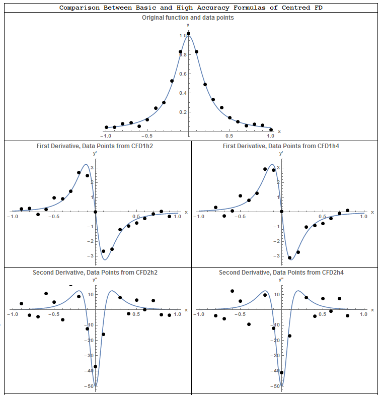
The following tool draws the plots of the exact first, second, third, and fourth derivatives of the Runge function overlaid with the data points of the first, second, third, and fourth derivatives obtained using the basic formulas for the forward, backward, and centred finite difference. Choose and notice the following: in general, the centred finite difference scheme provides more accurate results, especially for the second and third derivatives. For all the formulas, accuracy is lost with the higher derivatives especially in the neighbourhood of where the function and its derivatives have large variations within a small region. The forward finite difference uses the function information on the right of the point to calculate the derivative and hence the calculated derivatives appear to be slightly shifted to the left in comparison with the exact derivatives. This is evident when looking at any of the derivatives. Similarly, the backward finite difference uses the function information on the left of the point to calculate the derivative and hence the calculated derivatives appear to be slightly shifted to the right in comparison with the exact derivatives. The centred finite difference scheme does not exhibit the same behaviour because it uses the information from both sides. When choosing , the formulas provide very good approximation with the exact derivatives almost exactly overlaid with the finite difference calculations. However, for , the results of the finite difference calculations for the higher derivatives are far from accurate in the neighbourhood of for the third and fourth derivatives.

Choose and notice that for the first derivative using forward finite difference, the derivative for the last point is unavailable (why?). Similarly, using the backward finite difference, the derivative for the first point is unavailable. The derivatives for the first and last points are unavailable if the centred finite difference scheme is used. This carries on for the higher derivatives with the second, third, and fourth derivatives being unavailable for the last two, three, and four points when the forward finite difference scheme is used. The situation is reversed for the backward finite difference. The centred finite difference scheme provides more balanced results. The first and second derivatives at the first and last points are unavailable while the third and fourth derivatives at the first two points and the last two points are unavailable.

Higher Accuracy Formulas

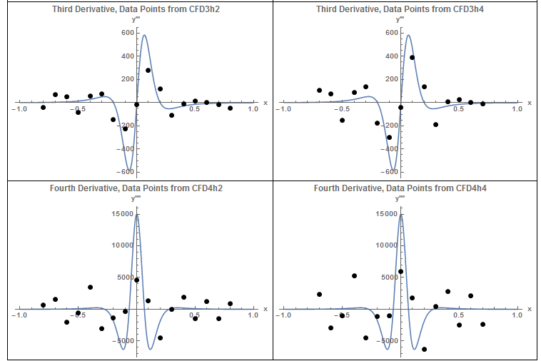
The observations from the basic formulas carry over to the higher accuracy formulas except that the results are unavailable at a larger number of points on the edges of the domain. Choose and notice that the first derivative is unavailable at the last two points because the forward finite difference higher accuracy formulas use the information at to calculate the derivative at . Similarly, the first derivative is unavailable at the first two points in the backward finite difference higher accuracy formulas because the scheme uses the information at to calculate the derivative at . For higher derivatives, more results are unavailable at a larger number of points close to the edge of the domain. Similar to the basic formulas scheme, the centred finite difference provides more balanced results with the results being unavailable at the points on both edges of the domain.

Forward Finite Difference

Both the basic formulas, and higher accuracy formulas for the forward finite difference scheme provide similar results. For , both schemes provide very good approximations for the first derivative, and for the flat parts of the higher derivatives. As explained above, the derivatives calculated using the formulas appear to be shifted to the left in comparison to the actual derivatives. For , both schemes provide relatively accurate predictions.

Backward Finite Difference

Both the basic formulas, and higher accuracy formulas for the backward finite difference scheme provide similar results. For , both schemes provides very good approximations for the first derivative, and for the flat parts of the higher derivatives. As explained above, the derivatives calculated using the formulas appear to be shifted to the right in comparison to the actual derivatives. For , both schemes provide relatively accurate predictions.

Centred Finite Difference

When , except for the fourth derivative at both centred finite difference schemes provide predictions that are very close to the exact results. It is obvious from these figures that when is relatively large, a centred finite difference scheme is perhaps more appropriate as it is more balanced and provides better accuracy. For smaller values of , all the schemes provide relatively acceptable predictions.

Derivatives Using Interpolation Functions

The basic and high-accuracy formulas derived above were based on equally spaced data, i.e., the distance between the points is constant. It is possible to derive formulas for unequally spaced data such that the derivatives would be a function of the spacings close to . Another method is to fit a piecewise interpolation function of a particular order to the data and then calculate its derivative as described previously. This technique in fact provides better estimates for higher values of as shown in the following tools. However, the disadvantage is that depending on the order of the interpolation function, higher derivatives are not available.

First Order Interpolation

The first order interpolation provides results for the first derivatives that are exactly similar to the results using forward finite difference. However, a first order interpolation function predicts zero second and higher derivatives. In the following tool, defines the interval at which the Runge function is sampled. The first derivative is calculated similar to the forward finite difference method. The higher derivatives are zero. The tool overlays the actual derivative with that predicted using the interpolation function. The black dots provide the values of the derivatives at the sampled points.

Second Order Interpolation

The second order interpolation provides much better results for compared with the finite difference formulas. However, the third and fourth derivatives are equal to zero. Change the value of to see its effect on the results.

Third Order Interpolation

The third order interpolation (cubic splines) provides much better results for compared with the finite difference formulas. However, the fourth derivative is equal to zero. Change the value of to see its effect on the results.

The following Mathematica code can be used to generate the tools above.
View Mathematica Code

h = 0.2;
n = 2/h + 1;
y = 1/(1 + 25 x^2);
yp = D[y, x];
ypp = D[yp, x];
yppp = D[ypp, x];
ypppp = D[yppp, x];
Data = Table[{-1 + h*(i - 1), (y /. x -> -1 + h*(i - 1))}, {i, 1, n}];
y2 = Interpolation[Data, Method -> "Spline", InterpolationOrder -> 1];
ypInter = D[y2[x], x];
yppInter = D[y2[x], {x, 2}];
ypppInter = D[y2[x], {x, 3}];
yppppInter = D[y2[x], {x, 4}];
Data1 = Table[{Data[[i, 1]], (ypInter /. x -> Data[[i, 1]])}, {i, 1,     n}];
Data2 = Table[{Data[[i, 1]], (yppInter /. x -> Data[[i, 1]])}, {i, 1,    n}];
Data3 = Table[{Data[[i, 1]], (ypppInter /. x -> Data[[i, 1]])}, {i, 1,    n}];
Data4 = Table[{Data[[i, 1]], (yppppInter /. x -> Data[[i, 1]])}, {i,    1, n}];
a0 = Plot[{y, y2[x]}, {x, -1, 1},   Epilog -> {PointSize[Large], Point[Data]}, AxesLabel -> {"x", "y"},  BaseStyle -> Bold, ImageSize -> Medium, PlotRange -> All,  PlotLegends -> {"y actual", "y spline"},    PlotLabel -> "First order splines"];
a1 = Plot[{yp, ypInter}, {x, -1, 1},    Epilog -> {PointSize[Large], Point[Data1]},    AxesLabel -> {"x", "y'"}, BaseStyle -> Bold, ImageSize -> Medium,    PlotRange -> All, PlotLegends -> {"y'", "y'spline"},    PlotLabel -> "First derivative"];
a2 = Plot[{ypp, yppInter}, {x, -1, 1},    Epilog -> {PointSize[Large], Point[Data2]},    AxesLabel -> {"x", "y''"}, BaseStyle -> Bold, ImageSize -> Medium,    PlotRange -> All, PlotLegends -> {"y''", "y''spline"},    PlotLabel -> "Second derivative"];
a3 = Plot[{yppp, ypppInter}, {x, -1, 1},    Epilog -> {PointSize[Large], Point[Data3]},    AxesLabel -> {"x", "y''"}, BaseStyle -> Bold, ImageSize -> Medium,    PlotRange -> All, PlotLegends -> {"y'''", "y'''spline"},    PlotLabel -> "Third derivative"];
a4 = Plot[{ypppp, yppppInter}, {x, -1, 1},    Epilog -> {PointSize[Large], Point[Data4]},    AxesLabel -> {"x", "y''"}, BaseStyle -> Bold, ImageSize -> Medium,    PlotRange -> All, PlotLegends -> {"y''''", "y''''spline"},    PlotLabel -> "Fourth derivative"];
Grid[{{a0}, {a1}, {a2}, {a3}, {a4}}]

Effect of Data Errors

One of the major problems when numerically differentiating empirical data is the existence of random (measurement) errors within the data itself. These errors cause the experimental data to have some natural fluctuations. If the experimental data is supposed to follow a particular model, then the best way to deal with such data is to find the best fit and use the derivatives of the best fit as described in the curve fitting section. However, if such a model does not exist, for example when measuring the position function of a moving subject, then care has to be taken when dealing with higher derivatives of the data. In particular, the fluctuations are magnified when higher derivatives are calculated.

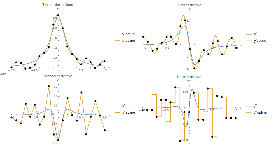
The following figures were generated by first sampling the Runge function on the domain at an interval of , then a random number between -0.1 and 0.1 is added to the data points. A cubic spline is then fit into the data. The small fluctuations in the data lead to very high fluctuations in all the derivatives. In particular, the second and third derivatives do not provide any useful information.

Clear[x]
h = 0.1;
n = 2/h + 1;
y = 1/(1 + 25 x^2);
yp = D[y, x];
ypp = D[yp, x];
yppp = D[ypp, x];
ypppp = D[yppp, x];
Data = Table[{-1 + h*(i - 1), (y /. x -> -1 + h*(i - 1)) +RandomReal[{-0.1, 0.1}]}, {i, 1, n}];
y2 = Interpolation[Data, Method -> "Spline", InterpolationOrder -> 3];
ypInter = D[y2[x], x];
yppInter = D[y2[x], {x, 2}];
ypppInter = D[y2[x], {x, 3}];
yppppInter = D[y2[x], {x, 4}];
Data1 = Table[{Data[[i, 1]], (ypInter /. x -> Data[[i, 1]])}, {i, 1, n}];
Data2 = Table[{Data[[i, 1]], (yppInter /. x -> Data[[i, 1]])}, {i, 1,n}];
Data3 = Table[{Data[[i, 1]], (ypppInter /. x -> Data[[i, 1]])}, {i, 1, n}];
Data4 = Table[{Data[[i, 1]], (yppppInter /. x -> Data[[i, 1]])}, {i, 1, n}];
a0 = Plot[{y, y2[x]}, {x, -1, 1}, Epilog -> {PointSize[Large], Point[Data]}, AxesLabel -> {"x", "y"}, BaseStyle -> Bold, ImageSize -> Medium, PlotRange -> All, PlotLegends -> {"y actual", "y spline"},  PlotLabel -> "Third order splines"];
a1 = Plot[{yp, ypInter}, {x, -1, 1}, Epilog -> {PointSize[Large], Point[Data1]}, AxesLabel -> {"x", "y'"}, BaseStyle -> Bold, ImageSize -> Medium, PlotRange -> All, PlotLegends -> {"y'", "y'spline"},  PlotLabel -> "First derivative"];
a2 = Plot[{ypp, yppInter}, {x, -1, 1}, Epilog -> {PointSize[Large], Point[Data2]}, AxesLabel -> {"x", "y''"}, BaseStyle -> Bold, ImageSize -> Medium,  PlotRange -> All, PlotLegends -> {"y''", "y''spline"},   PlotLabel -> "Second derivative"];
a3 = Plot[{yppp, ypppInter}, {x, -1, 1},    Epilog -> {PointSize[Large], Point[Data3]},    AxesLabel -> {"x", "y'''"}, BaseStyle -> Bold, ImageSize -> Medium,    PlotRange -> All, PlotLegends -> {"y'''", "y'''spline"},    PlotLabel -> "Third derivative"];
a4 = Plot[{ypppp, yppppInter}, {x, -1, 1},    Epilog -> {PointSize[Large], Point[Data4]},    AxesLabel -> {"x", "y''''"}, BaseStyle -> Bold, ImageSize -> Medium,    PlotRange -> All, PlotLegends -> {"y''''", "y''''spline"},    PlotLabel -> "Fourth derivative"];
Grid[{{a0,a1}, {a2,a3}}]

Similarly, the shown figures show the results when random numbers between -0.05 and 0.05 are added to the sampled data of the Runge function. When the centred finite difference scheme is used, the errors lead to very large variations in the second and third derivatives. The fourth derivative does not provide any useful information.

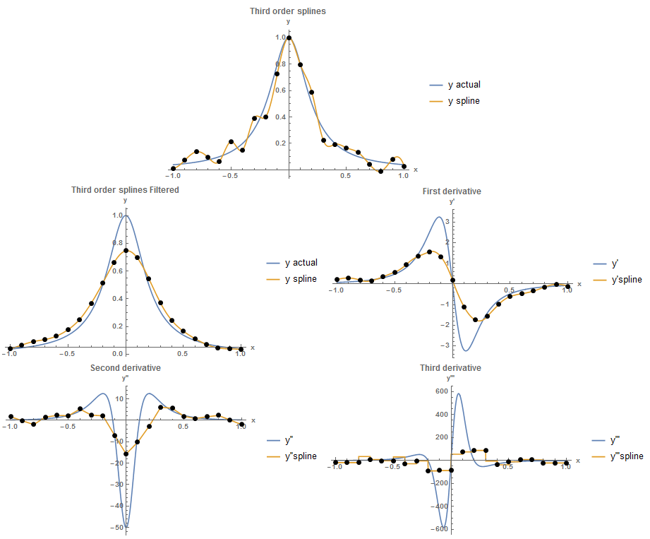
One possible solution to reduce noise in the data is to use a “Filter” to smooth the data. In the following figure, the built-in Gaussian Filter in Mathematica is used to reduce the generated noise. The fluctuations in the data are reduced and smoother derivatives are obtained.

View Mathematica Code

Clear[x]
h = 0.1;
n = 2/h + 1;
y = 1/(1 + 25 x^2);
yp = D[y, x];
ypp = D[yp, x];
yppp = D[ypp, x];
ypppp = D[yppp, x];
Data = Table[{-1 + h*(i - 1), (y /. x -> -1 + h*(i - 1)) +    RandomReal[{-0.1, 0.1}]}, {i, 1, n}];
Dataa = Data;
f = Data[[All, 2]];
f = GaussianFilter[f, 3];
Data = Table[{Data[[i, 1]], f[[i]]}, {i, 1, n}];
yun = Interpolation[Dataa, Method -> "Spline",   InterpolationOrder -> 3];
y2 = Interpolation[Data, Method -> "Spline", InterpolationOrder -> 3];
ypInter = D[y2[x], x];
yppInter = D[y2[x], {x, 2}];
ypppInter = D[y2[x], {x, 3}];
yppppInter = D[y2[x], {x, 4}];
Data1 = Table[{Data[[i, 1]], (ypInter /. x -> Data[[i, 1]])}, {i, 1,  n}];
Data2 = Table[{Data[[i, 1]], (yppInter /. x -> Data[[i, 1]])}, {i, 1, n}];
Data3 = Table[{Data[[i, 1]], (ypppInter /. x -> Data[[i, 1]])}, {i, 1, n}];
Data4 = Table[{Data[[i, 1]], (yppppInter /. x -> Data[[i, 1]])}, {i, 1, n}];
aun = Plot[{y, yun[x]}, {x, -1, 1}, Epilog -> {PointSize[Large], Point[Dataa]}, AxesLabel -> {"x", "y"}, BaseStyle -> Bold, ImageSize -> Medium, PlotRange -> All, PlotLegends -> {"y actual", "y spline"}, PlotLabel -> "Third order splines"];
a0 = Plot[{y, y2[x]}, {x, -1, 1},    Epilog -> {PointSize[Large], Point[Data]}, AxesLabel -> {"x", "y"},    BaseStyle -> Bold, ImageSize -> Medium, PlotRange -> All,    PlotLegends -> {"y actual", "y spline"},    PlotLabel -> "Third order splines Filtered"];
a1 = Plot[{yp, ypInter}, {x, -1, 1},    Epilog -> {PointSize[Large], Point[Data1]},    AxesLabel -> {"x", "y'"}, BaseStyle -> Bold, ImageSize -> Medium,    PlotRange -> All, PlotLegends -> {"y'", "y'spline"},    PlotLabel -> "First derivative"];
a2 = Plot[{ypp, yppInter}, {x, -1, 1},    Epilog -> {PointSize[Large], Point[Data2]},    AxesLabel -> {"x", "y''"}, BaseStyle -> Bold, ImageSize -> Medium,    PlotRange -> All, PlotLegends -> {"y''", "y''spline"},    PlotLabel -> "Second derivative"];
a3 = Plot[{yppp, ypppInter}, {x, -1, 1},    Epilog -> {PointSize[Large], Point[Data3]},    AxesLabel -> {"x", "y'''"}, BaseStyle -> Bold, ImageSize -> Medium,    PlotRange -> All, PlotLegends -> {"y'''", "y'''spline"},    PlotLabel -> "Third derivative"];
a4 = Plot[{ypppp, yppppInter}, {x, -1, 1},    Epilog -> {PointSize[Large], Point[Data4]},    AxesLabel -> {"x", "y''''"}, BaseStyle -> Bold, ImageSize -> Medium,    PlotRange -> All, PlotLegends -> {"y''''", "y''''spline"},    PlotLabel -> "Fourth derivative"];
Grid[{{aun, SpanFromLeft}, {a0, a1}, {a2, a3}}]

Problems

1. Compare the basic formulas and the high-accuracy formulas to calculate the first and second derivatives of at with . Clearly indicate the order of the error term in the approximation used. Calculate the relative error in each case.
2. A plane is being tracked by radar, and data are taken every two seconds in polar coordinates and .
   

   Time (sec.)	200	202	204	206	208	210
   (rad)	0.75	0.72	0.70	0.68	0.67	0.66
   (m.)	5120	5370	5560	5800	6030	6240

   The vector expression in polar coordinates for the velocity and the acceleration are given by:

      

   Use the centred finite difference basic formulas to find the velocity and acceleration vectors at sec. as a function of the unit vectors and . Then, using the norm of the velocity and acceleration vectors describe the plane speed and the magnitude of its acceleration.

3. Fick’s first diffusion law states that:

      

   where is the mass transported per unit area and per unit time with units , is a constant called the diffusion coefficient given in , is the concentration given in and is the distance in . The law states that the mass transported per unit area and per unit time is directly proportional to the gradient of the concentration (with a negative constant of proportionality). Stated differently, it means that the molecules tend to move towards the area of less concentration. If the concentration of a pollutant in the pore waters of sediments underlying the lake is constant throughout the year and is measured to be:

   	0	1	3
   ,	0.06	0.32	0.6

   where is the interface between the lake and the sediment. By fitting a parabola to the data, estimate at . If the area of interface between the lake and the sediment is , and if , how much pollutant in would be transported into the lake over a period of one year?

4. The positions in m. of the left and right feet of two squash players (Ramy Ashour and Cameron Pilley) during an 8 second segment of their match in the North American Open in February 2013 are given in the excel sheet provided here. Using a centred finite difference scheme, compare the average and top speed and acceleration between the two players during that segment of the match. Similarly, using a parabolic spline interpolation function, compare the average and top speed and acceleration between the two players. Finally, compare with the average speed of walking for humans.