
Introduction to Numerical Analysis: Curve Fitting
Given a set of data  with
with  , curve fitting revolves around finding a mathematical model that can describe the relationship
  such that the prediction of the mathematical model would match, as closely as possible, the given data. There are two advantages to finding an appropriate mathematical model with a good fit. The first advantage is the reduction of the data as the mathematical model will often have much fewer parameters than the actual data. The second advantage is the characterization of the response which allows calculating
  for any value for the variable
  within the range of applicability of the model.
The first step in curve fitting is to assume a particular mathematical model that might fit the data. The second step is to find the mathematical model parameters that would minimize the sum of the squares of the errors between the model prediction and the data. In these pages we will first present linear regression, which is basically fitting data to a linear mathematical model. Then, we will present nonlinear regression, i.e., fitting data to nonlinear mathematical models.
Linear Regression
Given a set of data with , a linear model fit to this set of data has the form:
![\[ y(x)=ax+b \]](https://engcourses-uofa.ca/wp-content/ql-cache/quicklatex.com-478ab3df9bf33e860112c64faaa7e409_l3.png "Rendered by QuickLaTeX.com")
where  and
and  are the model parameters. The model parameters can be found by minimizing the sum of the squares of the difference (
 ) between the data points and the model predictions:
![\[ S=\sum_{i=1}^n\left(y(x_i)-y_i\right)^2 \]](https://engcourses-uofa.ca/wp-content/ql-cache/quicklatex.com-5ca818e66ef737a329d26ce586c1a6de_l3.png "Rendered by QuickLaTeX.com")
Substituting for  yields:
![\[ S=\sum_{i=1}^n\left(ax_i+b-y_i\right)^2 \]](https://engcourses-uofa.ca/wp-content/ql-cache/quicklatex.com-0e066f7f3e8dc243f53c5368164a7819_l3.png "Rendered by QuickLaTeX.com")
In order to minimize , we need to differentiate with respect to the unknown parameters and and set these two equations to zero:
![\[\begin{split} \frac{\partial S}{\partial a}&=2\sum_{i=1}^n\left(\left(ax_i+b-y_i\right)x_i\right)=0\\ \frac{\partial S}{\partial b}&=2\sum_{i=1}^n\left(ax_i+b-y_i\right)=0\\ \end{split} \]](https://engcourses-uofa.ca/wp-content/ql-cache/quicklatex.com-c86f27bdd62e54b9b8a48d4d00147ca0_l3.png "Rendered by QuickLaTeX.com")
Solving the above two equations yields the best linear fit to the data. The solution for and has the form:
![\[\begin{split} a&=\frac{n\sum_{i=1}^nx_iy_i-\sum_{i=1}^nx_i\sum_{i=1}^ny_i}{n\sum_{i=1}^nx_i^2-\left(\sum_{i=1}^nx_i\right)^2}\\ b&=\frac{\sum_{i=1}^ny_i-a\sum_{i=1}^nx_i}{n} \end{split} \]](https://engcourses-uofa.ca/wp-content/ql-cache/quicklatex.com-0a714803bbd34b662a3afd67ef3d2b7d_l3.png "Rendered by QuickLaTeX.com")
The built-in function “Fit” in mathematica can be used to find the best linear fit to any data. The following code illustrates the procedure to use “Fit” to find the equation of the line that fits the given array of data:
View Mathematica Code
Data = {{1, 0.5}, {2, 2.5}, {3, 2}, {4, 4.0}, {5, 3.5}, {6, 6.0}, {7,  5.5}};
y = Fit[Data, {1, x}, x]
Plot[y, {x, 1, 7}, Epilog -> {PointSize[Large], Point[Data]}, AxesLabel -> {"x", "y"}, AxesOrigin -> {0, 0}]
Coefficient of Determination
The coefficient of determination, denoted  or
or  and pronounced
  squared, is a number that provides a statistical measure of how the produced model fits the data. The value of can be calculated as follows:
![\[ R^2=1-\frac{\sum_{i=1}^n\left(y_i-y(x_i)\right)^2}{\sum_{i=1}^n\left(y_i-\frac{1}{n}\sum_{i=1}^ny_i\right)^2} \]](https://engcourses-uofa.ca/wp-content/ql-cache/quicklatex.com-cb17c5ebbb39c9535ffeebca15081ed2_l3.png "Rendered by QuickLaTeX.com")
The equation above implies that  . A value closer to 1 indicates that the model is a good fit for the data while a value of 0 indicates that the model does not fit the data.
Using Mathematica and/or Excel
The built-in Mathematica function “LinearModelFit” provides the statistical measures associated with a linear regression model, including the confidence intervals in the parameters and . However, these are not covered in this course. The “LinearModelFit” can be used to output the of the linear fit as follows:
View Mathematica Code
Data = {{1, 0.5}, {2, 2.5}, {3, 2}, {4, 4.0}, {5, 3.5}, {6, 6.0}, {7, 5.5}};
y2 = LinearModelFit[Data, x, x]
y = Normal[y2]
y3 = y2["RSquared"]
Plot[y, {x, 1, 7}, Epilog -> {PointSize[Large], Point[Data]}, AxesLabel -> {"x", "y"}, AxesOrigin -> {0, 0}]
The following user-defined Mathematica procedure finds the linear fit and and draws the curve for a set of data:
View Mathematica Code
Clear[a, b, x]
Data = {{1, 0.5}, {2, 2.5}, {3, 2}, {4, 4.0}, {5, 3.5}, {6, 6.0}, {7, 5.5}};
LinearFit[Data_] :=
 (n = Length[Data];
  a = (n*Sum[Data[[i, 1]]*Data[[i, 2]], {i, 1, n}] - Sum[Data[[i, 1]], {i, 1, n}]*Sum[Data[[i, 2]], {i, 1, n}])/(n*Sum[Data[[i, 1]]^2, {i, 1, n}] - (Sum[Data[[i, 1]], {i, 1, n}])^2);
  b=(Sum[Data[[i, 2]], {i, 1, n}] - a*Sum[Data[[i, 1]], {i, 1, n}])/    n;
   RSquared=1-Sum[(Data[[i,2]]-a*Data[[i,1]]-b)^2,{i,1,n}]/Sum[(Data[[i,2]]-1/n*Sum[Data[[j,2]],{j,1,n}])^2,{i,1,n}];
  {RSquared,a,b })
LinearFit[Data]
RSquared=LinearFit[Data][[1]]
a = LinearFit[Data][[2]]
b = LinearFit[Data][[3]]
y = a*x + b;
Plot[y, {x, 1, 7}, Epilog -> {PointSize[Large], Point[Data]}, AxesLabel -> {"x", "y"}, AxesOrigin -> {0, 0} ]
Microsoft Excel can be used to provide the linear fit (linear regression) for any set of data. First, the curve is plotted using “XY scatter”. Afterwards, right clicking on the data curve and selecting “Add Trendline” will provide the linear fit. You can format the trendline to “show equation on chart” and .
Example
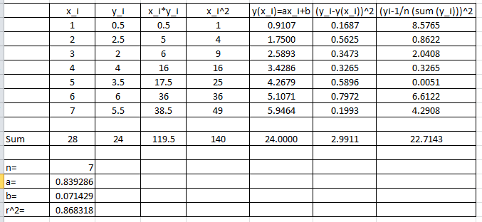
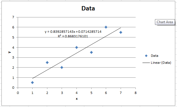
Find the best linear fit to the data (1,0.5), (2,2.5), (3,2), (4,4), (5,3.5), (6,6), (7,5.5).
Solution
Using the equations for , , and :
![\[ \begin{split} a&=\frac{n\sum_{i=1}^nx_iy_i-\sum_{i=1}^nx_i\sum_{i=1}^ny_i}{n\sum_{i=1}^nx_i^2-\left(\sum_{i=1}^nx_i\right)^2}=\frac{7(119.5)-(28)(24)}{7(140)-(28)^2}=0.839286\\ b&=\frac{\sum_{i=1}^ny_i-a\sum_{i=1}^nx_i}{n}=\frac{24-(0.839286)(28)}{7}=0.071429\\ R^2&=1-\frac{\sum_{i=1}^n\left(y_i-y(x_i)\right)^2}{\sum_{i=1}^n\left(y_i-\frac{1}{n}\sum_{i=1}^ny_i\right)^2}=1-\frac{2.9911}{22.7143}=0.8683 \end{split} \]](https://engcourses-uofa.ca/wp-content/ql-cache/quicklatex.com-9d8471a88231edf93598501efa25c307_l3.png "Rendered by QuickLaTeX.com")
Microsoft Excel can easily be used to generate the values for , , and as shown in the following sheet
The following is the Microsoft Excel chart produced as described above.
Extension of Linear Regression
In the previous section, the model function was linear in . However, we can have a model function that is linear in the unknown coefficients but non-linear in . In a general sense, the model function can be composed of  terms with the following form:
![\[ y(x)=a_1f_1(x)+a_2f_2(x)+a_3f_3(x)+\cdots+a_mf_m(x)=\sum_{j=1}^ma_jf_j(x) \]](https://engcourses-uofa.ca/wp-content/ql-cache/quicklatex.com-fcbcd0fe201a142feda736f1afbe018c_l3.png "Rendered by QuickLaTeX.com")
Note that the linear regression model can be viewed as a special case of this general form with only two functions  and
and  . Another special case of this general form is polynomial regression where the model function has the form:
![\[ y(x)=a_0+a_1x+a_2x^2+a_3x^3+\cdots+a_mx^m \]](https://engcourses-uofa.ca/wp-content/ql-cache/quicklatex.com-562efe1d633ccb47e3e38ef73f738699_l3.png "Rendered by QuickLaTeX.com")
The regression procedure constitutes finding the coefficients  that would yield the least sum of squared differences between the data and model prediction. Given a set of data with , and if is the sum of the squared differences between a general linear regression model and the data, then has the form:
![\[ S=\sum_{i=1}^n\left(y(x_i)-y_i\right)^2=\sum_{i=1}^n\left(\sum_{j=1}^ma_jf_j(x_i)-y_i\right)^2 \]](https://engcourses-uofa.ca/wp-content/ql-cache/quicklatex.com-fa606167e913062b559ed2a6a01270bd_l3.png "Rendered by QuickLaTeX.com")
To find the minimizers of , the derivatives of with respect to each of the coefficients can be equated to zero. Taking the derivative of with respect to an arbitrary coefficient  and equating to zero yields the general equation:
![\[ \frac{\partial S}{\partial a_k}=\sum_{i=1}^n\left(2\left(\sum_{j=1}^ma_jf_j(x_i)-y_i\right)f_k(x_i)\right)=0 \]](https://engcourses-uofa.ca/wp-content/ql-cache/quicklatex.com-18bf836354b92f2f576f7b1f2ab06a29_l3.png "Rendered by QuickLaTeX.com")
A system of -equations of the unknowns  can be formed and have the form:
![\[ \begin{split} \left(\begin{matrix} \sum_{i=1}^nf_1(x_i)f_1(x_i)&\sum_{i=1}^nf_1(x_i)f_2(x_i)&\cdots & \sum_{i=1}^nf_1(x_i)f_m(x_i)\\ \sum_{i=1}^nf_2(x_i)f_1(x_i)&\sum_{i=1}^nf_2(x_i)f_2(x_i)&\cdots & \sum_{i=1}^nf_2(x_i)f_m(x_i)\\ \vdots&\vdots&\ddots & \vdots\\ \sum_{i=1}^nf_m(x_i)f_1(x_i)&\sum_{i=1}^nf_m(x_i)f_2(x_i)&\cdots & \sum_{i=1}^nf_m(x_i)f_m(x_i) \end{matrix}\right)&\left(\begin{array}{c}a_1\\a_2\\\vdots\\a_m\end{array}\right)\\ &= \left(\begin{array}{c}\sum_{i=1}^ny_if_1(x_i)\\\sum_{i=1}^ny_if_2(x_i)\\\vdots\\\sum_{i=1}^ny_if_m(x_i)\end{array}\right) \end{split} \]](https://engcourses-uofa.ca/wp-content/ql-cache/quicklatex.com-b1c79ca30fa9cb87832dbf416da9edcb_l3.png "Rendered by QuickLaTeX.com")
It can be shown that the above system always has a unique solution when the functions  are non-zero and distinct. Solving these equations yields the best fit to the data, i.e., the best coefficients
  that would minimize the sum of the squares of the differences between the model and the data. The coefficient of determination can be obtained as described above.
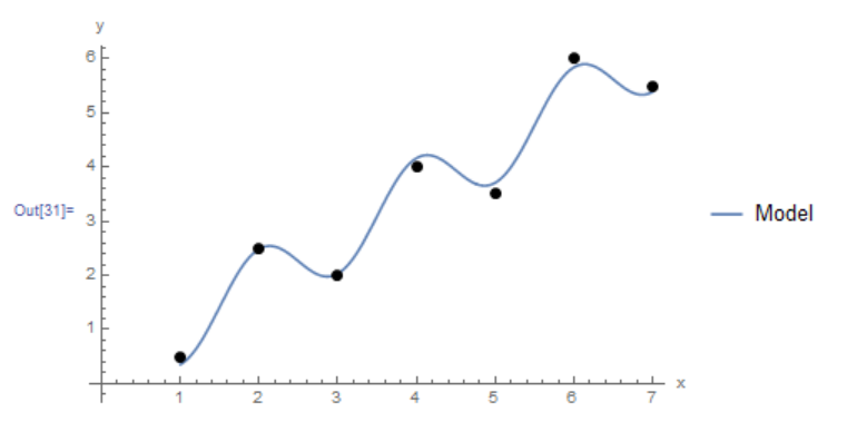
Example 1
Consider the data (1,0.5), (2,2.5), (3,2), (4,4), (5,3.5), (6,6), (7,5.5). Consider a model of the form
![\[ y=a_1+a_2x+a_3 \cos{(\pi x)} \]](https://engcourses-uofa.ca/wp-content/ql-cache/quicklatex.com-a4c55b2f0c1b988fc7e077e2adbe4e72_l3.png "Rendered by QuickLaTeX.com")
Find the coefficients  ,
,  , and
, and  that would give the best fit.
Solution
This model is composed of a linear combination of three functions: , , and  . To find the best coefficients, the following linear system of equations needs to be solved:
![\[ \begin{split} \left(\begin{matrix} \sum_{i=1}^nf_1(x_i)f_1(x_i)&\sum_{i=1}^nf_1(x_i)f_2(x_i)& \sum_{i=1}^nf_1(x_i)f_3(x_i)\\ \sum_{i=1}^nf_2(x_i)f_1(x_i)&\sum_{i=1}^nf_2(x_i)f_2(x_i)&\sum_{i=1}^nf_2(x_i)f_3(x_i)\\ \sum_{i=1}^nf_3(x_i)f_1(x_i)&\sum_{i=1}^nf_3(x_i)f_2(x_i)&\sum_{i=1}^nf_3(x_i)f_3(x_i) \end{matrix}\right)&\left(\begin{array}{c}a_1\\a_2\\a_3\end{array}\right)\\ &= \left(\begin{array}{c}\sum_{i=1}^ny_if_1(x_i)\\\sum_{i=1}^ny_if_2(x_i)\\\sum_{i=1}^ny_if_3(x_i)\end{array}\right) \end{split} \]](https://engcourses-uofa.ca/wp-content/ql-cache/quicklatex.com-97a4096cdfad0c845674190bc43e0f27_l3.png "Rendered by QuickLaTeX.com")
The following Microsoft Excel table is used to calculate the entries in the above matrix equation
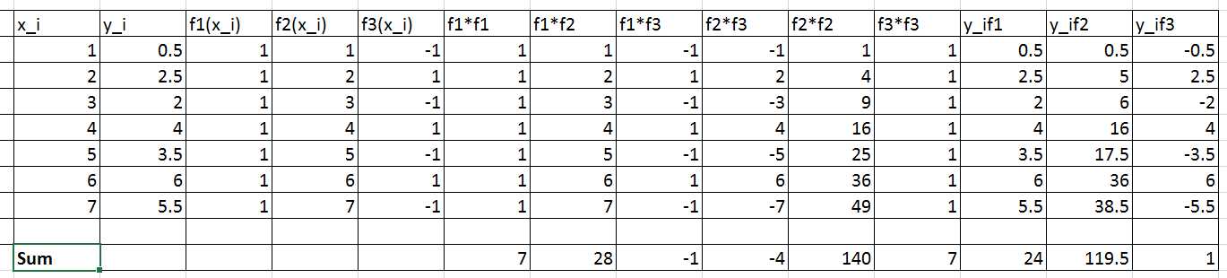
Therefore, the linear system of equations can be written as:
![\[ \left(\begin{matrix} 7&28&-1\\ 28&140&-4\\ -1&-4&7 \end{matrix}\right) \left(\begin{array}{c}a_1\\a_2\\a_3\end{array}\right)= \left(\begin{array}{c}24\\119.5\\1\end{array}\right) \]](https://engcourses-uofa.ca/wp-content/ql-cache/quicklatex.com-b7e97b875a8306b1df2aee29e336211f_l3.png "Rendered by QuickLaTeX.com")
Solving the above system yields  ,
,  ,
,  . Therefore, the best-fit model has the form:
![\[ y(x)=0.16369+0.83929x+0.64583\cos{(\pi x)} \]](https://engcourses-uofa.ca/wp-content/ql-cache/quicklatex.com-41790bcbbcbcf2389422feaa19daf8ec_l3.png "Rendered by QuickLaTeX.com")
To find the coefficient of determination, the following Microsoft Excel table for the values of  and
and  is used:
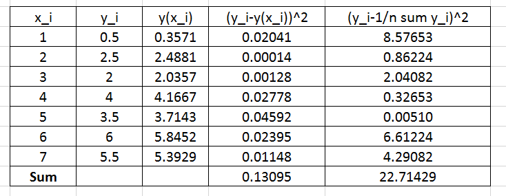
Therefore:
![\[ R^2=1-\frac{0.13095}{22.71429}=0.994234 \]](https://engcourses-uofa.ca/wp-content/ql-cache/quicklatex.com-c262dbe31fccfa0cb607109f9a2b98ef_l3.png "Rendered by QuickLaTeX.com")
is very close to 1 indicating a very good fit!
The Mathematica function LinearModelFit[Data,{functions},x] does the above computations and provides the required model. The equation of the model can be retrieved using the built-in function Normal and the can also be retrieved as shown in the code below. The final plot of the model vs. the data is shown below as well.
View Mathematica Code
Clear[a, b, x]
Data = {{1, 0.5}, {2, 2.5}, {3, 2}, {4, 4.0}, {5, 3.5}, {6, 6.0}, {7, 5.5}};
model = LinearModelFit[Data, {1, x, Cos[Pi*x]}, x]
y = Normal[model]
R2 = model["RSquared"]
Plot[y, {x, 1, 7}, Epilog -> {PointSize[Large], Point[Data]},  PlotLegends->{"Model"},AxesLabel -> {"x", "y"}, AxesOrigin -> {0, 0} ]
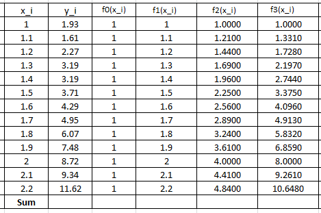
Example 2
Fit a cubic polynomial to the data (1,1.93),(1.1,1.61),(1.2,2.27),(1.3,3.19),(1.4,3.19),(1.5,3.71),(1.6,4.29),(1.7,4.95),(1.8,6.07),(1.9,7.48),(2,8.72),(2.1,9.34),(2.2,11.62).
Solution
A cubic polynomial fit would have the form:
![\[ y(x)=a_0+a_1x+a_2x^2+a_3x^3 \]](https://engcourses-uofa.ca/wp-content/ql-cache/quicklatex.com-2df5db35281a1a852627a77cf1d61218_l3.png "Rendered by QuickLaTeX.com")
This is a linear combination of the functions  ,
,  ,
,  , and
, and  . The following system of equations needs to be formed to solve for the coefficients
  , , , and :
![\[ \begin{split} \left(\begin{matrix} \sum_{i=1}^nf_0(x_i)f_0(x_i)&\sum_{i=1}^nf_0(x_i)f_1(x_i)&\sum_{i=1}^nf_0(x_i)f_2(x_i) & \sum_{i=1}^nf_0(x_i)f_3(x_i)\\ \sum_{i=1}^nf_1(x_i)f_0(x_i)&\sum_{i=1}^nf_1(x_i)f_1(x_i)&\sum_{i=1}^nf_1(x_i)f_2(x_i) & \sum_{i=1}^nf_1(x_i)f_3(x_i)\\ \sum_{i=1}^nf_2(x_i)f_0(x_i)&\sum_{i=1}^nf_2(x_i)f_1(x_i)&\sum_{i=1}^nf_2(x_i)f_2(x_i) & \sum_{i=1}^nf_2(x_i)f_3(x_i)\\ \sum_{i=1}^nf_3(x_i)f_0(x_i)&\sum_{i=1}^nf_3(x_i)f_1(x_i)&\sum_{i=1}^nf_3(x_i)f_2(x_i) & \sum_{i=1}^nf_3(x_i)f_3(x_i)\\ \end{matrix}\right)&\left(\begin{array}{c}a_0\\a_1\\a_2\\a_3\end{array}\right)\\ &= \left(\begin{array}{c}\sum_{i=1}^ny_if_0(x_i)\\\sum_{i=1}^ny_if_1(x_i)\\\sum_{i=1}^ny_if_2(x_i)\\\sum_{i=1}^ny_if_3(x_i)\end{array}\right) \end{split} \]](https://engcourses-uofa.ca/wp-content/ql-cache/quicklatex.com-15c52b52117fe39050710d5ef1b30979_l3.png "Rendered by QuickLaTeX.com")
The following Microsoft Excel tables are used to find the entries of the above linear system of equations:
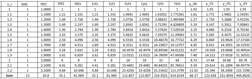
Therefore, the linear system of equations can be written as:
![\[ \left(\begin{matrix} 13&20.8&35.1&61.984\\ 20.8&35.1&61.984&113.607\\ 35.1&61.984&113.607&214.502\\ 61.984&113.607&214.502&414.623 \end{matrix}\right)\left(\begin{array}{c}a_0\\a_1\\a_2\\a_3\end{array}\right)= \left(\begin{array}{c}68.37\\123.638\\231.4056\\444.8628\end{array}\right) \]](https://engcourses-uofa.ca/wp-content/ql-cache/quicklatex.com-38b4a3d502bbf78de66f888077e07cea_l3.png "Rendered by QuickLaTeX.com")
Solving the above system yields  ,
,  ,
,  , and
, and  . Therefore, the best-fit model has the form:
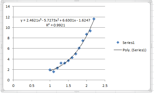
![\[ y=-1.6247+6.6301x-5.7273x^2+2.46212x^3 \]](https://engcourses-uofa.ca/wp-content/ql-cache/quicklatex.com-86a6f417d92ccf2c81cb73cb0b0ff0d8_l3.png "Rendered by QuickLaTeX.com")
The following graph shows the Microsoft Excel plot with the generated cubic trendline. The trendline equation generated by Excel is the same as the one above.
To find the coefficient of determination, the following Microsoft Excel table for the values of and is used:
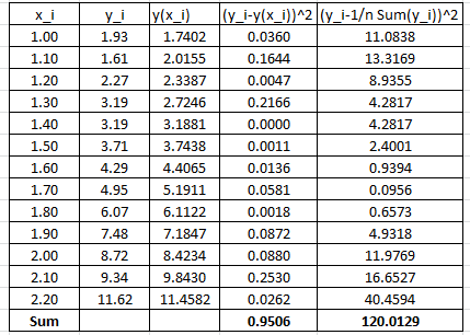
Therefore:
![\[ R^2=1-\frac{0.9506}{120.0129}=0.9921 \]](https://engcourses-uofa.ca/wp-content/ql-cache/quicklatex.com-8d56542a012847468b53122af9214a57_l3.png "Rendered by QuickLaTeX.com")
Which is similar to the one produced by Microsoft Excel. Alternatively, the following Mathematica code does the above computations to produce the model and its .
Data = {{1, 1.93}, {1.1, 1.61}, {1.2, 2.27}, {1.3, 3.19}, {1.4,3.19}, {1.5, 3.71}, {1.6, 4.29}, {1.7, 4.95}, {1.8, 6.07}, {1.9,7.48}, {2, 8.72}, {2.1, 9.34}, {2.2, 11.62}};
model = LinearModelFit[Data, {1, x, x^2, x^3}, x]
y = Normal[model]
R2 = model["RSquared"]
Plot[y, {x, 1, 2.2}, Epilog -> {PointSize[Large], Point[Data]}, PlotLegends -> {"Model"}, AxesLabel -> {"x", "y"}, AxesOrigin -> {0, 0} ]
Linearization of Nonlinear Relationships
In the previous two sections, the model function was formed as a linear combination of functions  and the minimization of the sum of the squares of the differences between the model prediction and the data produced a linear system of equations to solve for the coefficients in the model. In that case was linear in the coefficients. In certain situations, it is possible to convert nonlinear relationships to a linear form similar to the previous methods. For example, consider the following models
  ,
,  , and
, and  :
:
![\[ y_{\mbox{exp}}=b_1e^{a_1x}\qquad y_{\mbox{power}}=b_2x^{a_2} \qquad y_{\mbox{log}}=a_3\ln x + b_3 \]](https://engcourses-uofa.ca/wp-content/ql-cache/quicklatex.com-73a7cc21269e7c7bbe53ec123dd9ce9f_l3.png "Rendered by QuickLaTeX.com")
is an exponential model, is a power model, while is a logarithmic model. These models are nonlinear in and the unknown coefficients. However, by taking the natural logarithm of the first two, they can easily be transformed into linear models as follows:
![\[ \ln y_{\mbox{exp}}=a_1 x+\ln b_1 \qquad \ln y_{\mbox{power}}=a_2 \ln x+\ln b_2 \]](https://engcourses-uofa.ca/wp-content/ql-cache/quicklatex.com-70c38065963bfedd01df189565583fa8_l3.png "Rendered by QuickLaTeX.com")
In the first model, the data can be converted to  and linear regression can be used to find the coefficients and
  . For the second model, the data can be converted to
  and linear regression can be used to find the coefficients , and
  . The third model can be considered linear after converting the data into the form
  .
.
Coefficient of Determination for Nonlinear Relationships
For nonlinear relationships, the coefficient of determination is not a very good measure for how well the data fit the model. See for example this article on the subject. In fact, different software will give different values for . We will use the coefficient of determination for nonlinear relationships defined as:
![\[ R^2=1-\frac{\sum_{i=1}^n\left(y_i-y(x_i)\right)^2}{\sum_{i=1}^n\left(y_i\right)^2} \]](https://engcourses-uofa.ca/wp-content/ql-cache/quicklatex.com-3663cd85879c1a7697fb6cdc50fd095d_l3.png "Rendered by QuickLaTeX.com")
which is equal to 1 minus the ratio between the model sum of squares and the total sum of squares of the data. This is consistent with the definition of used in Mathematica for nonlinear models.
Example 1
Fit an exponential model to the data: (1,1.93),(1.1,1.61),(1.2,2.27),(1.3,3.19),(1.4,3.19),(1.5,3.71),(1.6,4.29),(1.7,4.95),(1.8,6.07),(1.9,7.48),(2,8.72),(2.1,9.34),(2.2,11.62).
Solution
The exponential model has the form:
![\[ y_{\mbox{exp}}=b_1e^{a_1x} \]](https://engcourses-uofa.ca/wp-content/ql-cache/quicklatex.com-f5e48e11bfab6bcdbc9c79b4dda0f5e3_l3.png "Rendered by QuickLaTeX.com")
This form can be linearized as follows:
![\[ \ln y_{\mbox{exp}}=a_1 x+\ln b_1 \]](https://engcourses-uofa.ca/wp-content/ql-cache/quicklatex.com-2bfc84d3f71df1f15ac122ee8ff93bec_l3.png "Rendered by QuickLaTeX.com")
The data needs to be converted to .  will be used to designate
  . The following Microsoft Excel table shows the raw data, and after conversion to
  .
.
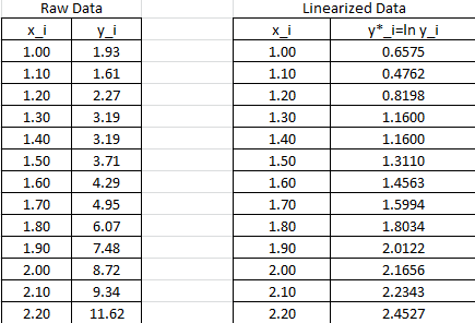
The linear regression described above will be used to find the best fit for the model:
![\[ y^*=a^*x+b^* \]](https://engcourses-uofa.ca/wp-content/ql-cache/quicklatex.com-79d70094716fbb4e77a2f429563ae743_l3.png "Rendered by QuickLaTeX.com")
with
![\[\begin{split} a^*&=\frac{n\sum_{i=1}^nx_iy^*_i-\sum_{i=1}^nx_i\sum_{i=1}^ny^*_i}{n\sum_{i=1}^nx_i^2-\left(\sum_{i=1}^nx_i\right)^2}\\ b^*&=\frac{\sum_{i=1}^ny^*_i-a^*\sum_{i=1}^nx_i}{n} \end{split} \]](https://engcourses-uofa.ca/wp-content/ql-cache/quicklatex.com-9a9f5fab4ff7894f00b478917a9be950_l3.png "Rendered by QuickLaTeX.com")
The following Microsoft Excel table is used to calculate the various entries in the above equation:
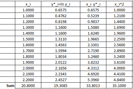
Therefore:
![\[\begin{split} a^*&=\frac{13\times 33.8013-20.8\times 19.3085}{13\times 35.10-\left(20.8\right)^2}=1.5976\\ b^*&=\frac{19.3085-1.5976\times 20.8}{13}=-1.0709 \end{split} \]](https://engcourses-uofa.ca/wp-content/ql-cache/quicklatex.com-9ef5f1ec81ef86268def7a3574ab826b_l3.png "Rendered by QuickLaTeX.com")
These can be used to calculate the coefficients in the original model:
![\[ a_1=a^*=1.5976 \qquad b_1=e^{b^*}=e^{-1.0709}=0.3427 \]](https://engcourses-uofa.ca/wp-content/ql-cache/quicklatex.com-f5cf7d668275b0f1f0283d83562c622b_l3.png "Rendered by QuickLaTeX.com")
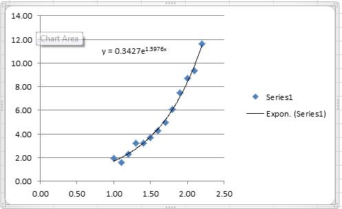
Therefore, the best exponential model based on the least squares of the linearized version has the form:
![\[ y_{\mbox{exp}}=0.3427e^{1.5976x} \]](https://engcourses-uofa.ca/wp-content/ql-cache/quicklatex.com-785cea551d11abbcbb865bf07e428820_l3.png "Rendered by QuickLaTeX.com")
The following Microsoft Excel chart shows the calculated trendline in Excel with the same coefficients:
It is possible to calculate the coefficient of determination for the linearized version of this model, however, it would only describe how good the linearized model is. For the nonlinear model, we will use the coefficient of determination as described above which requires the following Microsoft Excel table:
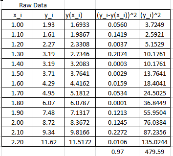
In this case, the coefficient of determination can be calculated as:
![\[ R^2=1-\frac{\sum_{i=1}^n\left(y_i-y(x_i)\right)^2}{\sum_{i=1}^n\left(y_i\right)^2}=1-\frac{0.97}{479.59}=0.998 \]](https://engcourses-uofa.ca/wp-content/ql-cache/quicklatex.com-d7ef59a652d688c8964334d07d78010f_l3.png "Rendered by QuickLaTeX.com")
The NonlinearModelFit built-in function in Mathematica can be used to generate the model and calculate its as shown in the code below.
View Mathematica Code
Data = {{1, 1.93}, {1.1, 1.61}, {1.2, 2.27}, {1.3, 3.19}, {1.4, 3.19}, {1.5, 3.71}, {1.6, 4.29}, {1.7, 4.95}, {1.8, 6.07}, {1.9, 7.48}, {2, 8.72}, {2.1, 9.34}, {2.2, 11.62}};
model = NonlinearModelFit[Data, b1*E^(a1*x), {a1, b1}, x]
y = Normal[model]
R2 = model["RSquared"]
Plot[y, {x, 1, 2.2}, Epilog -> {PointSize[Large], Point[Data]}, PlotLegends -> {"Model"}, AxesLabel -> {"x", "y"}, AxesOrigin -> {0, 0} ]
Example 2
Fit a power model to the data: (1,1.93),(1.1,1.61),(1.2,2.27),(1.3,3.19),(1.4,3.19),(1.5,3.71),(1.6,4.29),(1.7,4.95),(1.8,6.07),(1.9,7.48),(2,8.72),(2.1,9.34),(2.2,11.62).
Solution
The power model has the form:
![\[ y_{\mbox{power}}=b_2x^{a_2} \]](https://engcourses-uofa.ca/wp-content/ql-cache/quicklatex.com-af1e0999e1db65c780a86137ffb21392_l3.png "Rendered by QuickLaTeX.com")
This form can be linearized as follows:
![\[ \ln y_{\mbox{power}}=a_2 \ln x+\ln b_2 \]](https://engcourses-uofa.ca/wp-content/ql-cache/quicklatex.com-125f9fcf2879da77a2e1ae5134e6cbf4_l3.png "Rendered by QuickLaTeX.com")
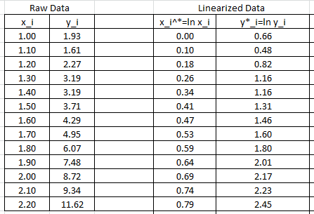
The data needs to be converted to . and  will be used to designate and
  respectively. The following Microsoft Excel table shows the raw data, and after conversion to
  .
.
The linear regression described above will be used to find the best fit for the model:
![\[ y^*=a^*x^*+b^* \]](https://engcourses-uofa.ca/wp-content/ql-cache/quicklatex.com-e9d81742385d3a72ce4228bfaadce433_l3.png "Rendered by QuickLaTeX.com")
with
![\[\begin{split} a^*&=\frac{n\sum_{i=1}^nx_i^*y^*_i-\sum_{i=1}^nx_i^*\sum_{i=1}^ny^*_i}{n\sum_{i=1}^n(x_i^*)^2-\left(\sum_{i=1}^nx_i^*\right)^2}\\ b^*&=\frac{\sum_{i=1}^ny^*_i-a^*\sum_{i=1}^nx_i^*}{n} \end{split} \]](https://engcourses-uofa.ca/wp-content/ql-cache/quicklatex.com-a29951a9d7ef796b61d592d4c08c5bb4_l3.png "Rendered by QuickLaTeX.com")
The following Microsoft Excel table is used to calculate the various entries in the above equation:
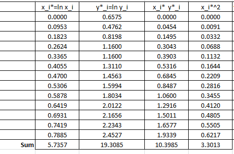
Therefore:
![\[\begin{split} a^*&=\frac{13\times 10.3985-5.7357\times 19.3085}{13\times 3.3013-\left(5.7357\right)^2}=2.4387\\ b^*&=\frac{19.3085-2.4387\times 5.7357}{13}=0.4093 \end{split} \]](https://engcourses-uofa.ca/wp-content/ql-cache/quicklatex.com-a983518a266e2135410359310577a6de_l3.png "Rendered by QuickLaTeX.com")
These can be used to calculate the coefficients in the original model:
![\[ a_2=a^*=2.4387 \qquad b_2=e^{b^*}=e^{0.4093}=1.5058 \]](https://engcourses-uofa.ca/wp-content/ql-cache/quicklatex.com-bd781e4867379495bfc0bebc1932e9d4_l3.png "Rendered by QuickLaTeX.com")
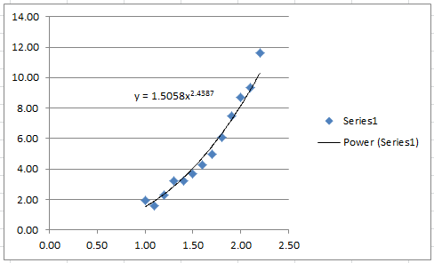
Therefore, the best power model based on the least squares of the linearized version has the form:
![\[ y_{\mbox{power}}=1.5058x^{2.4387} \]](https://engcourses-uofa.ca/wp-content/ql-cache/quicklatex.com-fc68ca1b4c214e163d898a7d3aadd0c8_l3.png "Rendered by QuickLaTeX.com")
The following Microsoft Excel chart shows the calculated trendline in Excel with the same coefficients:
It is possible to calculate the coefficient of determination for the linearized version of this model, however, it would only describe how good the linearized model is. For the nonlinear model, we will use the coefficient of determination as described above which requires the following Microsoft Excel table:
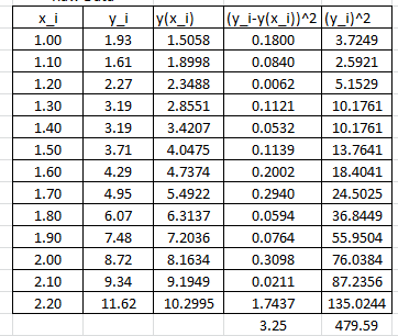
In this case, the coefficient of determination can be calculated as:
![\[ R^2=1-\frac{\sum_{i=1}^n\left(y_i-y(x_i)\right)^2}{\sum_{i=1}^n\left(y_i\right)^2}=1-\frac{3.25}{479.59}=0.9932 \]](https://engcourses-uofa.ca/wp-content/ql-cache/quicklatex.com-be917fc971daf446a7ee2b40a0ca2b70_l3.png "Rendered by QuickLaTeX.com")
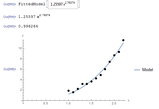
The NonlinearModelFit built-in function in Mathematica can be used to generate a slightly better model with a higher as shown in the code below.
View Mathematica Code
Data = {{1, 1.93}, {1.1, 1.61}, {1.2, 2.27}, {1.3, 3.19}, {1.4, 3.19}, {1.5, 3.71}, {1.6, 4.29}, {1.7, 4.95}, {1.8, 6.07}, {1.9, 7.48}, {2, 8.72}, {2.1, 9.34}, {2.2, 11.62}};
model = NonlinearModelFit[Data, b1*x^(a1), {a1, b1}, x]
y = Normal[model]
R2 = model["RSquared"]
Plot[y, {x, 1, 2.2}, Epilog -> {PointSize[Large], Point[Data]}, PlotLegends -> {"Model"}, AxesLabel -> {"x", "y"}, AxesOrigin -> {0, 0} ]
The following is the corresponding Mathematica output
Nonlinear Regression
In nonlinear regression, the model function is a nonlinear function of and of the parameters  . Given a set of
  data points with , curve fitting starts by assuming a model with parameters. The parameters can be obtained by minimizing the least squares:
![\[ S=\sum_{i=1}^n (y(x_i)-y_i)^2 \]](https://engcourses-uofa.ca/wp-content/ql-cache/quicklatex.com-387790132f7cd8137334ae64f3d7a94e_l3.png "Rendered by QuickLaTeX.com")
In order to find the parameters of the model that would minimize , equations of the following form are solved:
![\[ \frac{\partial S}{\partial a_k}=\sum_{i=1}^n\left(2\left(y(x_i)-y_i\right)\frac{\partial y}{\partial a_k}\bigg|_{x=x_i}\right)=0 \]](https://engcourses-uofa.ca/wp-content/ql-cache/quicklatex.com-14189d72a2bd6f2e05a2b5eb0c261a3a_l3.png "Rendered by QuickLaTeX.com")
Since is nonlinear in the coefficients, the equations formed are also nonlinear and can only be solved using a nonlinear equation solver method such as the Newton Raphson method described before. We are going to rely on the built-in NonlinearModelFit function in Mathematica that does the required calculations.
Example 1
The following data describes the yield strength  and the plastic strain
  obtained from uniaxial experiments where the first variable is the plastic strain and the second variable is the corresponding yield strength: (0.0001,204.18),(0.0003,226.4),(0.0015,270.35),(0.0025,276.86),(0.004,296.86),(0.005,299.3),(0.015,334.65),(0.025,346.56),(0.04,371.81),(0.05,377.45),(0.1,398.01),(0.15,422.45),(0.2,434.42).
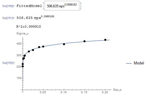
Use the NonlinearModelFit function in Mathematica to find the best fit for the data assuming the relationship follows the form:
![\[ \sigma_y=K\varepsilon_p^n \]](https://engcourses-uofa.ca/wp-content/ql-cache/quicklatex.com-ca2ae54f65e70a6ac3555edfdc3c7af2_l3.png "Rendered by QuickLaTeX.com")
Solution
While this model can be linearized as described in the previous section, the NonlinearModelFit will be used. The array of data is input as a list in the variable Data. The NonlinearModelFit function is then used and the output is stored in the variable: “model”. The form of the best fit function is evaluated using the built-in function Normal[model]. can be evaluated as well as shown in the code below. The values of  and that describe the best fit are
  and
and  . Therefore, the best-fit model is:
![\[ \sigma_y=506.64\varepsilon_p^{0.0988} \]](https://engcourses-uofa.ca/wp-content/ql-cache/quicklatex.com-78f714053b46580494713814e16c770a_l3.png "Rendered by QuickLaTeX.com")
The following is the Mathematica code used along with the output
View Mathematica Code
Data = {{0.0001, 204.18}, {0.0003, 226.4}, {0.0015, 270.35}, {0.0025, 276.86}, {0.004, 296.86}, {0.005, 299.3}, {0.015, 334.65}, {0.025,346.56}, {0.04, 371.81}, {0.05, 377.45}, {0.1, 398.01}, {0.15, 422.45}, {0.2, 434.42}};
model = NonlinearModelFit[Data, Kk*eps^(n), {Kk, n}, eps]
y = Normal[model]
Print["R^2=",R2 = model["RSquared"]]
Plot[y, {eps, 0, 0.21}, Epilog -> {PointSize[Large], Point[Data]}, PlotLegends -> {"Model"}, AxesLabel -> {"Eps_p", "Sigma_y"}, AxesOrigin -> {0, 0}]
Example 2
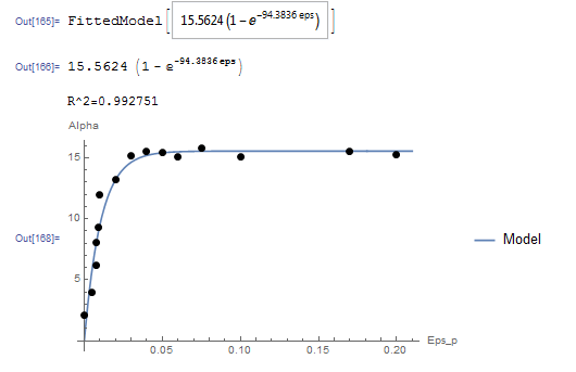
Exponential and Logarithmic Models offer a wide range of model functions that can be used for various engineering applications. An example is the exponential model that describes an initial rapid increase in the dependent variable which then levels off to become asymptotic to an upper limit :
![\[ y(x)=a_1(1-e^{-a_2x}) \]](https://engcourses-uofa.ca/wp-content/ql-cache/quicklatex.com-870c0424e00daf30910a88bd7f8e11e2_l3.png "Rendered by QuickLaTeX.com")
where and are the model parameters. For plastic materials, Armstrong and Frederick proposed this model in 1966 (republished here in 2007) to describe how a quantity called the “Centre of the Yield Surface” changes with the increase in the plastic strain. If  is the centre of the yield surface and is the plastic strain, then, the model for has the form:
![\[ \alpha = C\left(1-e^{-\gamma \varepsilon_p}\right) \]](https://engcourses-uofa.ca/wp-content/ql-cache/quicklatex.com-7f125f0e7ec7abdd3d6a73d6b6e85c3b_l3.png "Rendered by QuickLaTeX.com")
Find the values of  and
and  for the best fit to the experimental data
  given by: (0.0001,2.067),(0.005,3.96),(0.0075,6.22),(0.008,8.07),(0.009,9.32),(0.01,12.02),(0.02,13.2),(0.03,15.22),(0.04,15.51),(0.05,15.44),(0.06,15.1),(0.075,15.76),(0.1,15.11),(0.17,15.53),(0.2,15.26)
Solution
Unlike the model in the previous question, this model cannot be linearized. The NonlinearModelFit built-in function in Mathematica will be used. The array of data is input as a list in the variable Data. The NonlinearModelFit function is then used and the output is stored in the variable: “model”. The form of the best fit function is evaluated using the built-in function Normal[model]. can be evaluated as well as shown in the code below. The values of and that describe the best fit are  and
and  . Therefore, the best-fit model is:
![\[ \alpha = 15.5624\left(1-e^{-94.3836 \varepsilon_p}\right) \]](https://engcourses-uofa.ca/wp-content/ql-cache/quicklatex.com-9cac1d5b9daca0cb0f06f35edee174ee_l3.png "Rendered by QuickLaTeX.com")
The following is the Mathematica code used along with the output
View Mathematica CodeData = {{0.0001, 2.067}, {0.005, 3.96}, {0.0075, 6.22}, {0.008,8.07}, {0.009, 9.32}, {0.01, 12.02}, {0.02, 13.2}, {0.03,15.22}, {0.04, 15.51}, {0.05, 15.44}, {0.06, 15.1}, {0.075,15.76}, {0.1, 15.11}, {0.17, 15.53}, {0.2, 15.26}};
model = NonlinearModelFit[Data, Cc (1 - E^(-gamma*eps)), {Cc, gamma}, eps]
y = Normal[model]
Print["R^2=", R2 = model["RSquared"]]
Plot[y, {eps, 0, 0.21}, Epilog -> {PointSize[Large], Point[Data]}, PlotLegends -> {"Model"}, AxesLabel -> {"Eps_p", "Alpha"}, AxesOrigin -> {0, 0}]
Problems
- The following data provides the number of trucks with a particular weight at each hour of the day on one of the busy US highways. The data is provided as
 , where
  is the hour and
  is the number of trucks: (1,16),(2,12),(3,14),(4,8),(5,24),(6,92),(7,311),(8,243),(9,558),(10,644),(11,768),(12,838),(13,911),(14,897),(15,853),(16,860),(17,853),(18,875),(19,673),(20,378),(21,207),(22,142),(23,108),(24,62). The distribution follows a Gaussian model of the form:
![\[ N=a_1 e^{\frac{-(x-a_2)^2}{a_3}} \]](https://engcourses-uofa.ca/wp-content/ql-cache/quicklatex.com-84ff8075b23cdfbb09baba137c079d55_l3.png "Rendered by QuickLaTeX.com")
- Find the parameters , , and that would produce the best fit to the data.
- On the same plot draw the model prediction vs. the data.
- Calculate the of the model.
- Calculate the sum of squares of the difference between the model prediction and the data.
- Find the parameters
-
In 2014, MacLeans published the following table showing the average tuition in Canadian provinces for the period from 2010 to 2014.
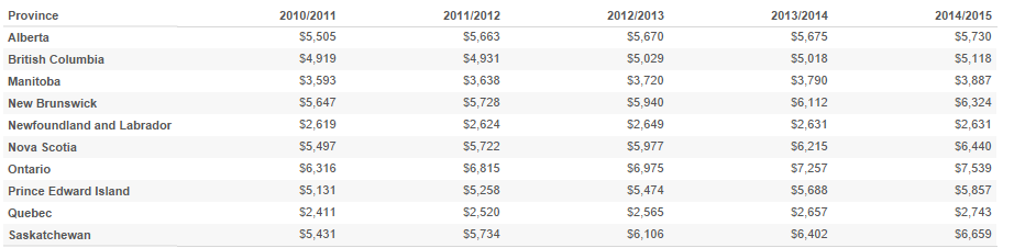
- Find the best linear model for each province that would predict tuition each year and its associated . Use calendar years to represent the axis data.
- Based on the linear fit, which province has the highest tuition increase per year and which one has the lowest?
- Find the best linear model for each province that would predict tuition each year and its associated
- The yield strength of steel decreases with elevated temperatures. The following experimental data provides the value of the temperature in 1000 degrees Celsius and the corresponding reduction factor in the yield strength. (0.05,1), (0.1,1), (0.2,0.95), (0.3,0.92), (0.4,0.82), (0.5,0.6), (0.6,0.4), (0.7,0.15), (0.8,0.15), (0.9,0.1), (1.0,0.1). Find the parameters
 in the following model that would provide the best fit to the data:
![\[ R=a_1+\frac{a_2}{1+a_3 e^{\left(a_4x+a_5\right)}} \]](https://engcourses-uofa.ca/wp-content/ql-cache/quicklatex.com-f935e14ba8fdfded4f6954ec26088186_l3.png "Rendered by QuickLaTeX.com")
Also, on the same plot draw the model prediction vs. the data. Based on the model, what is the reduction in the yield strength at temperatures of 150, 450, and 750 Degrees Celsius?
- In order to noninvasively assess the stability of medical implants, Westover et al. devised a technique by which the implant is struck using a hand-piece while measuring the acceleration response.
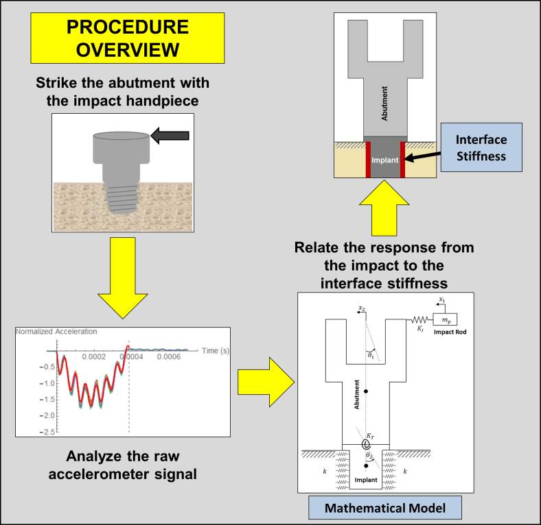 In order to assess the stability, the acceleration
  data as a function of time
  has to be fit to a model of the form:
![\[\begin{split} y(t)&=a_1\sin{(a_2t+\phi_1)}+a_3e^{-a_4a_5t}\sin{\left(\sqrt{\left(1-a_4^2\right)}a_5t+\phi_2\right)}\\ a(t)&=\frac{\mathrm{d}^2y(t)}{\mathrm{d}t^2} \end{split} \]](https://engcourses-uofa.ca/wp-content/ql-cache/quicklatex.com-f6ca6d05fdcbfc248b760a7ea16d6451_l3.png "Rendered by QuickLaTeX.com")
where
 is the position,
  is the acceleration, , , ,
  ,
,  ,
,  , and
, and  are the model parameters. Initial guesses for the model parameters can be taken as:
  respectively.
The following text file OneStrike.txt contains the acceleration data collected by striking one of the implants. Download the data file and use the NonLinearModelFit built-in function to calculate the parameters for the best-fit model along with the value of. Plot the data overlapping the model.Reference: L. Westover, W. Hodgetts, G. Faulkner, D. Raboud. 2015. Advanced System for Implant Stability Testing (ASIST). OSSEO 2015 5th International Congress on Bone Conduction Hearing and Related Technologies, Fairmont Chateau Lake Louise, Canada, May 20 – 23, 2015.
- Find the parabola
 that best fits the following data:
x 2.2 1.1 -0.11 -1.1 -2.2 y 6.38 -1.21 -4.18 -3.63 1.65 -
Find the exponential model that best fits the following data:
data = {{10, 5.7}, {20, 18.2}, {30, 44.3}, {40, 74.5}, {50, 130.2}} - Find the power model that best fits the following data:
data = {{10, 5.7}, {20, 18.2}, {30, 44.3}, {40, 74.5}, {50, 130.2}} -
Linear regression can be extended when the data depends on more than one variable (called multiple linear regression). For example, if the dependent variable is
 while the independent variables are and , then the data to be fitted have the form
  . In this case, the best-fit model is represented by a plane of the form
  . Using least squares assumption, find expressions for finding the coefficients of the model: , , and .