Engineering at Alberta Courses » Introduction and Graphical Methods

Finding Roots of Equations: Introduction and Graphical Methods

Let $f:[a,b]\rightarrow \mathbb{R}$ be a function. One of the most basic problems in numerical analysis is to find the value $x\in[a,b]$ that would render $f(x)=0$ . This value $x$ is called a root of the equation $f$ . As an example, consider the function $f(x)=2x-20$ . Consider the equation $f(x)=0$ . Clearly, there is only one root to this equation which is $x=10$ . Alternatively, consider $g:\mathbb{R}\rightarrow\mathbb{R}$ defined as $g(x)=a\times x^2+b\times x+c$ with $a,b,c\in\mathbb{R}$ . There are two analytical roots for the equation $g(x)=0$ given by

$x=\frac{-b\pm \sqrt{b^2-4ac}}{2a}$

In this section we are going to present three classes of methods: graphical, bracketing, and open methods for finding roots of equations.

Graphical Methods

Graphical methods rely on a computational device that calculates the values of the function along an interval at specific steps, and then draws the graph of the function. By visual inspection, the analyst can identify the points at which the function crosses the $x$ axis. Graphical methods are very useful for one-dimensional problems, but for multi-dimensional problems it is not possible to visualize a graph of a function of multi-variables.

Example

As an example, consider $f(x)=\sin{5x}+\cos{2x}$ . We wish to find the values of $x$ (i.e., the roots) that would satisfy the equation $f(x)=0$ for $x\in[-1,1]$ . The fastest way is to plot the graph (even Microsoft Excel would serve as an appropriate tool here) and then visually inspect the locations where the graph crosses the $x$ axis:

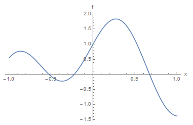
As shown in the above graph, the equation has three roots and just by visual inspection, the roots are around $x_1=-0.525$ , $x_2=-0.21$ , and $x_3=0.675$ . Of course these estimates are not that accurate for $f(x_1)=0.00365$ , $f(x_2)=0.0457$ , and $f(x_3)=-0.012$ . Whether these estimates are acceptable or not, depends on the requirements of the problem. We can further zoom in using the software to try and get better estimates:

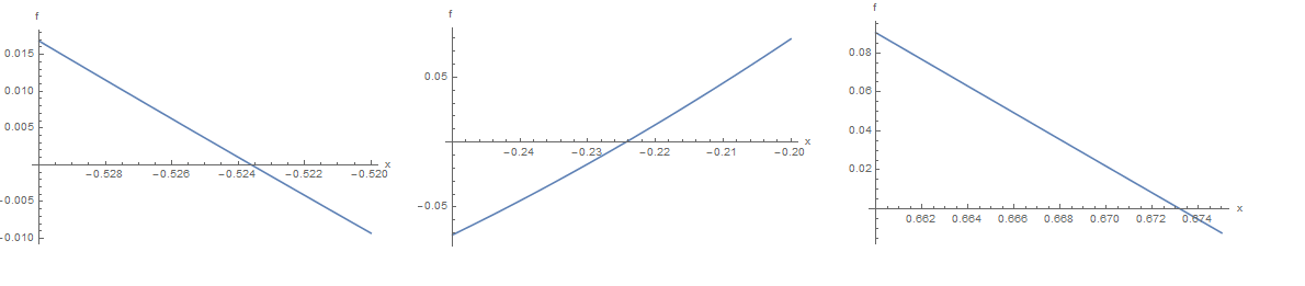
Visual inspection of the zoomed-in graphs provides the following estimates: $x_1=-0.5235$ , $x_2=-0.225$ , and $x_3=0.6731$ which are much better estimates since: $f(x_1)=0.00025$ , $f(x_2)=-0.0018$ , and $f(x_3)=0.00067$

View Mathematica Code

Clear[x]
f = Sin[5 x] + Cos[2 x]
Plot[f, {x, -1, 1}, AxesLabel -> {"x", "f"}]
f /. x -> -0.525
f /. x -> -0.21
f /. x -> 0.675
Plot[f, {x, -0.53, -0.52}, AxesLabel -> {"x", "f"}]
Plot[f, {x, -0.25, -0.2}, AxesLabel -> {"x", "f"}]
Plot[f, {x, 0.66, 0.675}, AxesLabel -> {"x", "f"}]
f /. x -> -0.5235
f /. x -> -0.225
f /. x -> 0.6731

View Python Code

import numpy as np
import matplotlib.pyplot as plt

def f(x): return np.sin(5*x) + np.cos(2*x)

x1 = np.arange(-1,1,0.01)
plt.plot(x1,f(x1))
plt.xlabel('x'); plt.ylabel('f')
plt.grid(); plt.show()

print("f(-0.525):",f(-0.525)) 
print("f(-0.21):",f(-0.21)) 
print("f(0.675):",f(0.675)) 

x2 = np.arange(-0.53, -0.52,0.01)
plt.plot(x2,f(x2))
plt.xlabel('x'); plt.ylabel('f')
plt.grid(); plt.show()

x3 = np.arange(-0.25, -0.2,0.01)
plt.plot(x3,f(x3))
plt.xlabel('x'); plt.ylabel('f')
plt.grid(); plt.show()

x4 = np.arange(0.66, 0.675,0.01)
plt.plot(x4,f(x4))
plt.xlabel('x'); plt.ylabel('f')
plt.grid(); plt.show()

print("f(-0.5235):",f(-0.5235)) 
print("f(-0.225):",f(-0.225)) 
print("f(0.6731):",f( 0.6731))

Open Educational Resources

Finding Roots of Equations: Introduction and Graphical Methods

Graphical Methods

Example

Leave a Reply Cancel reply