Engineering at Alberta Courses

Polynomial Interpolation: Introduction

Introduction to Polynomial Interpolation

Polynomial interpolation is the procedure of fitting a polynomial of degree $n$ to a set of $n+1$ data points. For example, if we have two data points, then we can fit a polynomial of degree 1 (i.e., a linear function) between the two points. If we have three data points, then we can fit a polynomial of the second degree (a parabola) that passes through the three points. Figure 1 shows fitting polynomials of degrees 1, 2, 3, and 4, to sets of 2, 3, 4, and 5 data points. The polynomial equation for each curve is shown in the title for each graph.

Polynomial interpolation relies on the fact that for every $n+1$ data points, there is a unique polynomial of degree $n$ that passes through these $n+1$ data points. This fact relies on the Fundamental Theorem of Algebra that states that every degree $n$ polynomial has exactly $n$ roots. So, if two degree $n$ polynomials $p_1$ and $p_2$ agree on $n+1$ points, then, their difference $z=p_1-p_2$ is a polynomial of degree $n$ but has $n+1$ roots which implies that $z=0$ .

To find the unique polynomial of degree $n$ that passes through $n+1$ data points, we need to solve a linear set of $n+1$ equations with the coefficients of the polynomial being the unknowns. Let $(x_i,y_i)$ be the $i^{th}$ data point where $i\leq n+1$ . Then, we have:

$\begin{split} a_0+a_1x_1+a_2x_1^2+\cdots +a_nx_1^n&=y_1\\ a_0+a_1x_2+a_2x_2^2+\cdots +a_nx_2^n&=y_2\\ &\vdots \\ a_0+a_1x_{n+1}+a_2x_{n+1}^2+\cdots +a_nx_{n+1}^n&=y_{n+1} \end{split}$

Which can be written as follows in matrix form:

(1) $\begin{equation*} \left(\begin{array}{ccccc}1&x_1&x_1^2&\cdots&x_1^n\\1&x_2&x_2^2&\cdots&x_2^n\\1&x_3&x_3^2&\cdots&x_3^n\\ \vdots&\vdots&\vdots&\vdots\\ 1&x_{n+1}&x_{n+1}^2&\cdots&x_{n+1}^n \end{array}\right)\left(\begin{array}{c}a_0\\a_1\\a_2\\\vdots\\a_n\end{array}\right)=\left(\begin{array}{c}y_1\\y_2\\y_3\\\vdots\\y_{n+1}\end{array}\right) \end{equation*}$

The above system can be solved to find the values of the coefficients $a_0,a_1,a_2,\cdots,a_n$ which would ensure that the polynomial curve $y=a_0+a_1x+a_2x^2+\cdots+a_nx^n$ passes through the $n+1$ data points.

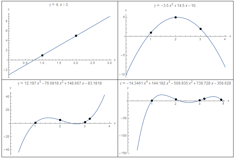
Figure 1. Polynomial Interpolation for 2, 3, 4, and 5 data points.

View Mathematica Code

Data = {{1, 1}, {2, 5.}};
y = InterpolatingPolynomial[Data, x];
a = Plot[y, {x, 0, 3}, Epilog -> {PointSize[Large], Point[Data]}, AxesLabel -> {"x", "y"}, ImageSize -> Medium, PlotLabel -> "y" == Expand[y]];

Data = {{1, 1}, {2, 5.}, {3, 2}};
y = InterpolatingPolynomial[Data, x];
b = Plot[y, {x, 0, 4}, Epilog -> {PointSize[Large], Point[Data]},AxesLabel -> {"x", "y"}, ImageSize -> Medium, PlotLabel -> "y" == Expand[y]];

Data = {{1, 1}, {2, 5}, {3, 2}, {3.2, 7}};
y = InterpolatingPolynomial[Data, x];
c = Plot[y, {x, 0, 4}, Epilog -> {PointSize[Large], Point[Data]}, AxesLabel -> {"x", "y"}, ImageSize -> Medium, PlotLabel -> "y" == Expand[y]];

Data = {{1, 1}, {2, 5}, {3, 2}, {3.2, 7}, {3.9, 4}};
y = InterpolatingPolynomial[Data, x];
d = Plot[y, {x, 0, 4}, Epilog -> {PointSize[Large], Point[Data]}, AxesLabel -> {"x", "y"}, ImageSize -> Medium, PlotLabel -> "y" == Expand[y]];
Grid[{{a, b}, {c, d}}, Frame -> All]

View Python Code

import numpy as np
import sympy as sp
import matplotlib.pyplot as plt

x = sp.symbols('x')
x_val = np.arange(0,4,0.01)

Data = [(1, 1), (2, 5.)]
y = sp.interpolate(Data, x)
plt.title(sp.N(y,3))
plt.plot(x_val, [y.subs(x,i) for i in x_val])
plt.scatter([point[0] for point in Data],[point[1] for point in Data], c='k')
plt.grid(); plt.show()

Data = [(1, 1), (2, 5.), (3, 2)]
y = sp.interpolate(Data, x)
plt.title(sp.N(y,3))
plt.plot(x_val, [y.subs(x,i) for i in x_val])
plt.scatter([point[0] for point in Data],[point[1] for point in Data], c='k')
plt.grid(); plt.show()

Data = [(1, 1), (2, 5), (3, 2), (3.2, 7)]
y = sp.interpolate(Data, x)
plt.title(sp.N(y,3))
plt.plot(x_val, [y.subs(x,i) for i in x_val])
plt.scatter([point[0] for point in Data],[point[1] for point in Data], c='k')
plt.grid(); plt.show()

Data = [(1, 1), (2, 5), (3, 2), (3.2, 7), (3.9, 4)]
y = sp.interpolate(Data, x)
plt.title(sp.N(y,3))
plt.plot(x_val, [y.subs(x,i) for i in x_val])
plt.scatter([point[0] for point in Data],[point[1] for point in Data], c='k')
plt.grid(); plt.show()

Example

Find an interpolating polynomial that would fit the data points $(1,1.1), (2,2.1), (3,5), (3.4,7)$ .

Solution

There are four data points, so, we can fit a third degree polynomial whose coefficients can be found by solving the following system of four linear equations:

$\left(\begin{matrix}1&1&1&1\\1&2&2^2&2^3\\1&3&3^2&3^3\\ 1&3.4&3.4^2&3.4^3 \end{matrix}\right)\left(\begin{array}{c}a_0\\a_1\\a_2\\a_3\end{array}\right)=\left(\begin{array}{c}1.1\\2.1\\5\\7\end{array}\right)$

Solving the above system yields:

$a_0=0.625\qquad a_1=0.670833\qquad a_2=-0.425 \qquad a_3=0.229167$

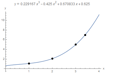
Therefore, the interpolating polynomial that would pass through all four data points is:

$y=0.625+0.670833x-0.425x^2+0.229167x^3$

The following Mathematica code was used to solve the above equations and produce the plot below:

View Mathematica Code

M = {{1, 1, 1, 1}, {1, 2, 4, 2^3}, {1, 3, 9, 27}, {1, 3.4, 3.4^2, 3.4^3}};
yv = {1.1, 2.1, 5, 7}
a = Inverse[M].yv
y = a[[1]] + a[[2]]*x + a[[3]]*x^2 + a[[4]]*x^3
Plot[y, {x, 0, 4}, Epilog -> {PointSize[Large],  Point[{{1, 1.1}, {2, 2.1}, {3, 5}, {3.4, 7}}]}, AxesLabel -> {"x", "y"}, ImageSize -> Medium, PlotLabel -> "y" == Expand[y]]

View Python Code

import numpy as np
import sympy as sp
import matplotlib.pyplot as plt

M = [[1, 1, 1, 1], [1, 2, 4, 2**3], [1, 3, 9, 27], [1, 3.4, 3.4**2, 3.4**3]]
yv = [1.1, 2.1, 5, 7]
a = np.matmul(np.linalg.inv(M),yv)
x = sp.symbols('x')
y = a[0] + a[1]*x + a[2]*x**2 + a[3]*x**3
x_val = np.arange(0,4,0.01)
plt.plot(x_val, [y.subs(x,i) for i in x_val])
plt.scatter([1, 2, 3, 3.4],[1.1, 2.1, 5, 7], c='k')
plt.title(sp.N(y,5))
plt.grid(); plt.show()

Interpolation2

MATLAB file: Download

Mathematica also has a built-in “InterpolatingPolynomial[Data,x]” function that would automatically form and solve the above equation as shown below. Simply provide the data points as a list and Mathematica would produce the interpolating polynomial as a function of “x”.

View Mathematica Code

Data = {{1, 1.1}, {2, 2.1}, {3, 5}, {3.4, 7}};
y = InterpolatingPolynomial[Data, x];
Plot[y, {x, 0, 4}, Epilog -> {PointSize[Large], Point[Data]}, AxesLabel -> {"x", "y"}, ImageSize -> Medium, PlotLabel -> "y" == Expand[y]]

View Python Code

import numpy as np
import sympy as sp
import matplotlib.pyplot as plt

x = sp.symbols('x')
Data = [(1, 1.1), (2, 2.1), (3, 5), (3.4, 7)]
y = sp.interpolate(Data, x)
x_val = np.arange(0,4,0.01)
plt.plot(x_val, [y.subs(x,i) for i in x_val])
plt.scatter([point[0] for point in Data],[point[1] for point in Data], c='k')
plt.title(sp.N(y,3))
plt.grid(); plt.show()

Disadvantages

There are various disadvantages to this interpolating polynomials method. The first disadvantage is that as the number of data points gets bigger, the linear systems of equations that need to be solved become ill-conditioned. In other words, the matrix that needs to be inverted would be composed of both small and very large numbers, a situation which is prone to round-off errors. Another major disadvantage is that as the number of data points increases, the order of the interpolating polynomial increases as well. By construction, the polynomial would pass through the data points. However, for large order ( $n>10$ ), the polynomial would be oscillating wildly between the data points leading to large errors in the interpolated values. The following example illustrates this:

Example

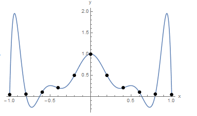
Consider the following 11 data points: (-1.00,0.038),(-0.80,0.058),(-0.60,0.100),(-0.4,0.200),(-0.20,0.500),(0.00,1.000),(0.20,0.500),(0.40,0.200),(0.60,0.100),(0.80,0.0580),(1.00,0.038). Using the InterpolatingPolynomial function in Mathematica the 10th order polynomial that would fit through all these points has the form:

$y=1-16.8551x^2+123.356x^4-381.407x^6+494.843x^8-220.9x^{10}$

From the plot below, the polynomial indeed passes through the 11 points, however, in between the points it oscillates wildly. In fact, for $0.8<x<1$ the values of the polynomial are much higher than the values at the points $x=0.8$ and $x=1$ which were used for the interpolation:
interpolation3

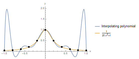
It is worth noting that the data points were actually generated using the Runge function:

$y=\frac{1}{1+25x^2}$

When $y$ is plotted versus the interpolation function, it is clear that the polynomial interpolation function, if used instead of $y$ would produce erroneous results for values outside of the control points. In fact, Runge used this example in the nineteenth century to show that using higher order polynomials to approximate functions does not always improve accuracy but can have detrimental effects on the values of the function in the intervals between the control points.
interpolation4

View Mathematica Code

Data = {{-1, 0.038}, {-0.8, 0.058}, {-0.60, 0.10}, {-0.4, 0.20}, {-0.2, 0.50}, {0, 1}, {0.2, 0.5}, {0.4, 0.2}, {0.6, 0.1}, {0.8, 0.058}, {1, 0.038}};
y = InterpolatingPolynomial[Data, x]
Chop[Expand[y]]
Plot[y, {x, -1, 1}, Epilog -> {PointSize[Large], Point[Data]}, AxesLabel -> {"x", "y"}, ImageSize -> Medium]
y2 = 1/(1 + 25 x^2)
Plot[{y, y2}, {x, -1, 1}, Epilog -> {PointSize[Large], Point[Data]}, AxesLabel -> {"x", "y"}, ImageSize -> Medium, PlotLegends -> {"Interpolating polynomial", y2}]

View Python Code

import numpy as np
import sympy as sp
import matplotlib.pyplot as plt

x = sp.symbols('x')
x_val = np.arange(-1,1.01,0.01)
Data = [(-1, 0.038), (-0.8, 0.058), (-0.60, 0.10), (-0.4, 0.20), (-0.2, 0.50), (0, 1), (0.2, 0.5), (0.4, 0.2), (0.6, 0.1), (0.8, 0.058), (1, 0.038)]
y = sp.interpolate(Data, x)
plt.plot(x_val, [y.subs(x,i) for i in x_val])
plt.scatter([point[0] for point in Data],[point[1] for point in Data], c='k')
plt.grid(); plt.show()

y2 = 1/(1 + 25*x**2)
plt.plot(x_val, [y.subs(x,i) for i in x_val], label='Interpolating polynomial')
plt.plot(x_val, [y2.subs(x,i) for i in x_val], label=y2)
plt.scatter([point[0] for point in Data],[point[1] for point in Data], c='k')
plt.legend(); plt.grid(); plt.show()

MATLAB file: Download

Open Educational Resources

Polynomial Interpolation: Introduction

Introduction to Polynomial Interpolation

Example

Solution

Disadvantages

Example

Lecture Video

Leave a Reply Cancel reply