Engineering at Alberta Courses » Introduction and Examples

Ordinary Differential Equations: Introduction and Examples

Ordinary Differential Equations (ODEs) are equations that relate the derivatives of one or more smooth functions with an independent variable $x\in\mathbb{R}$ . The term “ordinary” indicates that there is only one independent variable appearing in the equations.

Examples of Ordinary Differential Equations

ODEs appear naturally in almost all engineering applications. Here are some examples:

Newton’s Second Law of Motion

One of the most ubiquitously used ordinary differential equations is Newton’s second law of motion, which relates the second derivative of the position of a particle (i.e., the acceleration) to the applied force on the particle. The relationship has the form:

$m \frac{\mathrm{d}^2x}{\mathrm{d}t^2}=F(x,t)$

where $m$ is the mass of the particle. The time $t$ is the independent variable, while the dependent variable is the position $x(t)$ . Newton’s equation adopts different forms depending on the application. For example, to describe the free vibration of a spring-mass system with spring constant $k>0$ (Figure 1), then the equation has the form:

$m \frac{\mathrm{d}^2x}{\mathrm{d}t^2}+kx=0$

where $x$ is the position of the mass at the tip of the spring from the spring’s static equilibrium position.

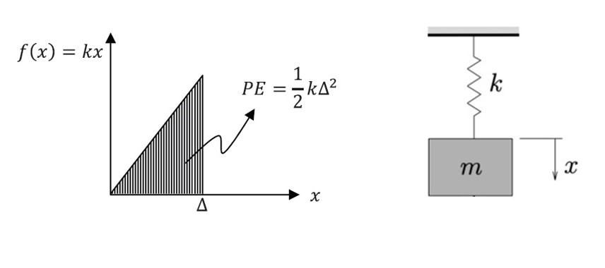
Figure 1. Mass-Linear Elastic Spring System

To clarify, assume a spring-mass system hung vertically. The forces acting on the mass are the spring force and the weight of the mass. The weight of the mass equals equals $mg$ where $g$ is the gravitational acceleration of the Earth. If $y$ denotes the (arbitrary) position of the mass measured from the unstretched length, $l_0$ , of the spring (Figure 2), the force by the spring equals $ky$ and the Newton’s second law of motion for the hung mass can be written as,

$m\frac{\mathrm d^2y}{\mathrm d^2t}=mg-ky$

The negative sign is due to the fact that the weight acts downward and the spring force acts upward when the spring is stretched as shown by the free body diagram in Figure 2.

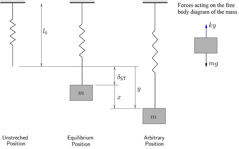
Figure 2. Spring-mass system.

At the static equilibrium (no vibration), the weight of the mass pulls the spring vertically down and initially gives the spring a constant stretch of $\delta_{ST} = mg/k$ . Therefore, $y$ can be written as $y=x+\delta_{ST}$ , where $x$ is the position of the mass with respect to the static equilibrium of the mass. Therefore, the above equation can be written as,

$\begin{split} m\frac{\mathrm d^2(x+\delta_{ST})}{\mathrm d^2t}&=mg-k(x+\delta_{ST})\\ m\frac{\mathrm d^2(x)}{\mathrm d^2t}&=-kx+mg-mg\\ \end{split}$

which leads to,

$m\frac{\mathrm d^2(x)}{\mathrm d^2t}+kx=0$

The explicit solution to this equation has the following form:

$x(t)=\frac{v_0}{\sqrt{k/m}}\sin\left(\sqrt{\frac{k}{m}t}\right)+x_0\cos\left(\sqrt{\frac{k}{m}t}\right)$

where $x_0$ and $v_0$ the initial position and initial velocity of the mass, and $\sqrt{k/m}$ is the natural frequency of the system (denoted as $p$ or $\omega_n$ ).

The displacement response of the system has the form shown in Figure 3.

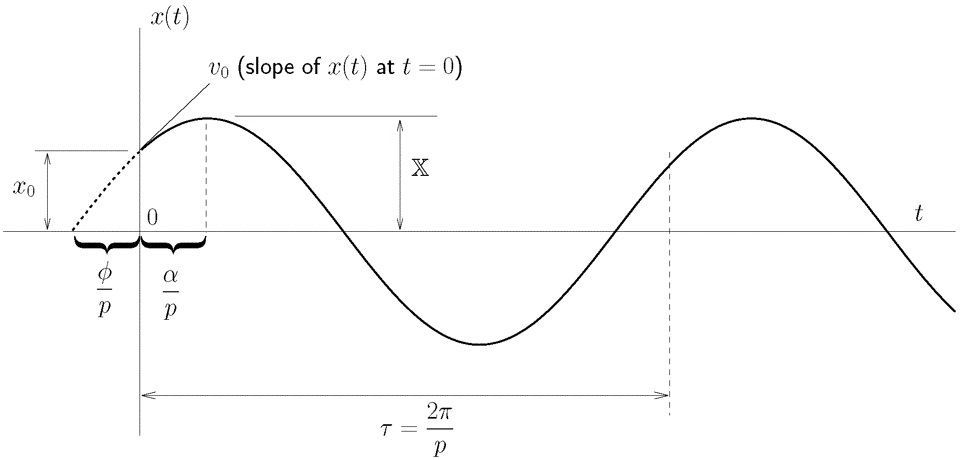
Figure 3. Free Vibration Response of a simple Mass-Spring System

If the external forces include a damping force (a force that is a function of the velocity and that is always opposite to the direction of motion), then, the equation has the form:

$m \frac{\mathrm{d}^2x}{\mathrm{d}t^2}+c\frac{\mathrm{d}x}{\mathrm{d}t}+kx=0$

where $c>0$ is the damping coefficient.

The explicit solution to this equation has the following form:

$x(t)=e^{-\zeta pt}\left[\frac{v_0+\zeta px_0}{\sqrt{1-\zeta^2p}}\sin\left(\sqrt{1-\zeta^2}pt\right)+x_0\cos\left(\sqrt{1-\zeta^2}pt\right)\right]$

where $\zeta$ is the damping ratio and $p=\sqrt{k/m}$ is the natural frequency of the system. Again $x_0$ and $v_0$ are the initial displacement and initial velocity of the mass, respectively.

The displacement response for the free vibration of a damped spring-mass system is shown in Figure 4.

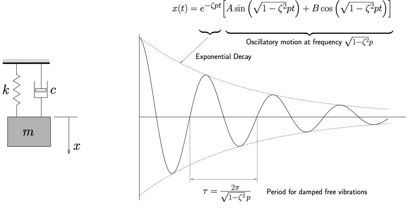
Figure 4. Left: Simple damped spring-mass system. Right: Free vibration response of a damped mass-spring system.

The following code utilizes the built-in DSolve function in Mathematica to solve the above simple equations. Also, the Manipulate built-in function is used to visualize the effect of varying $m$ and $k$ on the resulting vibration of the system.

View Mathematica Code

Clear[x, g, k, m]
(*General Solution*)
a = DSolve[m*x''[t] == - k*x[t] - beta*x'[t], x, t];
Print["General Solution (damped system)="]
x = x[t] /. a[[1]]

(*Solution*)
Clear[x, g, k, m, beta]
a = DSolve[{m*x''[t] == - k*x[t] - beta*x'[t], x[0] == 0, x'[0] == 0}, x, t];
Print["Solution with initial velocity and displacement =0"]
x = x[t] /. a[[1]];
x = Simplify[x]
Manipulate[g = 1;Graphics3D[{Cuboid[{-1, -1, -5}, {0, 0, -((E^(-(((beta + Sqrt[beta^2 - 4 k m]) t)/(2 m)))m (beta (-1 + E^((Sqrt[beta^2 - 4 k m] t)/m)) + (1 + E^((Sqrt[beta^2 - 4 k m] t)/m)-2 E^(((beta + Sqrt[beta^2 - 4 k m]) t)/(2 m))) Sqrt[beta^2 - 4 k m]))/(2 k Sqrt[beta^2 - 4 k m]))}]},  Axes -> True, PlotRange -> {{-1, 0}, {-1, 0}, {-5, 10}},  AxesOrigin -> {0, 0, 0}, ViewVertical -> {0, 0, -1}], {t, 0,  2*4*Pi*Sqrt[5]}, {m, 1, 5}, {beta, 0, 5}, {k, 1, 5}]

View Python Code

# UPGRADE: need Sympy 1.2 or later, upgrade by running: "!pip install sympy --upgrade" in a code cell
# !pip install sympy --upgrade
import cmath
import numpy as np
import sympy as sp
import matplotlib.pyplot as plt
from IPython.display import HTML
from ipywidgets.widgets import interact, Play
sp.init_printing(use_latex=True)
display(HTML('<link rel="stylesheet" href="//stackpath.bootstrapcdn.com/font-awesome/4.7.0/css/font-awesome.min.css"/>'))

x = sp.Function('x')
m, k, t, beta = sp.symbols('m k t beta')
# General Solution
sol = sp.dsolve(m*x(t).diff(t,2) + k*x(t) + beta*x(t).diff(t))
display("General Solution (damped system):", sol)

# Solution
sol = sp.dsolve(m*x(t).diff(t,2) + k*x(t) + beta*x(t).diff(t), ics={x(0): 0, x(t).diff(t).subs(t, 0): 0})
display("Solution with initial velocity and displacement = 0:", sp.simplify(sol))

@interact(t=Play(value=0, min=0, max=60, step=1, interval=500),
          m=(1,5,0.01), k=(1,5,0.01), beta=(0,5,0.01))
def update(t, m=1, k=1, beta=0):
  g = 1
  s = cmath.sqrt(beta**2 - 4*k*m)
  x = -((np.exp(-(((beta + s)*t)/(2*m)))*m*(beta*(-1 + np.exp((s*t)/m)) + (1 + np.exp((s*t)/m)-2*np.exp(((beta + s)*t)/(2*m)))*s))/(2*k*s))
  plt.xlim(0,10); plt.ylim(-0.1,0.1)
  plt.yticks([])
  plt.title('x = '+str(np.round(x,3)))
  plt.plot([0,x],[0,0],lw=50)

View Python Code

# Spring Animation

# UPGRADE: need Sympy 1.2 or later, upgrade by running: "!pip install sympy --upgrade" in a code cell
# !pip install sympy --upgrade
import numpy as np
import sympy as sp
import matplotlib.pyplot as plt
from IPython.display import HTML
from scipy.integrate import odeint
from matplotlib.patches import Rectangle
from ipywidgets.widgets import interact
display(HTML('<link rel="stylesheet" href="//stackpath.bootstrapcdn.com/font-awesome/4.7.0/css/font-awesome.min.css"/>'))

r = sp.Function('r')
t = sp.symbols('t')
x_val = np.arange(0,5,0.01)
@interact(displacement=(-0.1,0.1,0.05), velocity=(-1,1,0.05),
          mass=(5,10,0.05), damping_ratio=(0,1,0.01), stiffness=(200,750,1))
def update(displacement=0, velocity=0, mass=5, damping_ratio=0, stiffness=200):
  run  = 1
  cd = 1.5*(2*np.sqrt(stiffness*mass));
  w = np.sqrt(stiffness/(mass))
  w1 = w/(2*np.pi) 
  Tn = 1/w1
  U = (displacement + velocity)*Tn
  nt = run/Tn
  da = damping_ratio*cd
  sol = sp.dsolve(mass*r(t).diff(t,2) + da*r(t).diff(t) + stiffness*r(t), ics={r(0): displacement, r(t).diff(t).subs(t,0): velocity})
  l = sol.rhs.subs(t,run)
  
  plt.xlim(-1, 20)
  plt.ylim(-6, 6)
  plt.plot([-0.5,0,0],[0,0,2], 'k')
  plt.plot([3 + l, 3 + l, 4.5 + l],[-2, 0, 0], 'k')
  plt.plot([3*nx/11 + l*nx/11 for nx in range(12)], 
           [2*np.cos(np.pi*nx) for nx in range(12)], 'k')
  ax = plt.gca()
  ax.add_patch(Rectangle((-1,-6),0.5,12,color='black'))
  ax.add_patch(Rectangle((4.5 + l, -2),4,4,color='rosybrown'))
  plt.text(4,3,"f_n(Hz) = {}".format(round(w1,5)))
  plt.text(4,4,"T_n(s) = {}".format(round(Tn,5)))
  plt.show()

  plt.plot(x_val, [sol.rhs.subs(t,i) for i in x_val])
  plt.grid(); plt.show()

Beam Deflection

The deflection of an Euler-Bernoulli beam follows the following equation:

$EI\frac{\mathrm{d}^4y}{\mathrm{d}x^4}=q$

where $E$ is the beam’s Young’s modulus, $I$ is the cross sectional moment of inertia, $y$ is the beam’s deflection (the dependent variable), $q$ is the applied distributed load on the beam, and $x$ is the position along the beam’s length (the independent variable). For a fixed-ends beam; if the deflection and rotation at both ends of a beam of length $L$ is equal to zero, i.e. $y(0)=y(L)=y'(L)=y'(0)=0$ , and if $q$ is constant, then, the deflection of the beam has the form:

$y=\frac{qx^4-2Lqx^3+qL^2x^2}{24EI}$

Growth and Decay

If $x$ is the number of organisms at any time $t$ , and if the growth of the number depends on the number that is already there, then, the ODE that would describe this uninhibited growth is given by:

$\frac{\mathrm{d}x}{\mathrm{d}t}=kx$

Where $k>0$ is a positive constant. The time $t$ is the independent variable, while the dependent variable is the number of organisms $x(t)$ . The general solution of this equation has the form:

$x=C_1e^{kt}$

where $C_1$ is a constant depending on the boundary conditions. If the initial condition is such that $x(0)=A$ then, the solution has the form:

$x=Ae^{kt}$

Similarly, if rate of decrease (decay) of a quantity is a function of the amount available, then, the uninhibited decay can be described by the equation:

$\frac{\mathrm{d}y}{\mathrm{d}t}=-hy$

where $h>0$ is a positive constant. The time $t$ is the independent variable, while the dependent variable is the quantity $y(t)$ . Radioactive decay follows this ODE. The general solution of this equation has the form:

$y=C_1e^{-ht}$

where $C_1$ is a constant depending on the boundary conditions. If the initial condition is such that $y(0)=A$ then, the solution has the form:

$y=Ae^{-ht}$

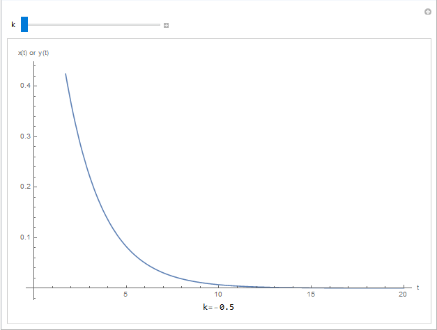
The following tool plots the quantities $x(t)$ or $y(t)$ when $A=1$ for different values of the exponent:

View Mathematica Code

Clear[x]
a = DSolve[x'[t] == k*x[t], x, t];
x = x[t] /. a[[1]]

Clear[x]
a = DSolve[{x'[t] == k*x[t], x[0] == A}, x, t]
x = x[t] /. a[[1]]

Manipulate[A = 1; r = Grid[{{"k=", k}}, Spacings -> 0]; Grid[{{Plot[A*E^(k*t), {t, 0, 20}, AxesLabel -> {"t", "x(t) or y(t)"}, ImageSize -> Medium]}, {r}}], {k, -0.5, 0.5}]

View Python Code

# UPGRADE: need Sympy 1.2 or later, upgrade by running: "!pip install sympy --upgrade" in a code cell
# !pip install sympy --upgrade
import numpy as np
import sympy as sp
import matplotlib.pyplot as plt
from ipywidgets.widgets import interact
sp.init_printing(use_latex=True)

x = sp.Function('x')
t, k, A = sp.symbols('t k A')
sol = sp.dsolve(x(t).diff(t) - k*x(t))
display(sol)
sol = sp.dsolve(x(t).diff(t) - k*x(t), ics={x(0): A})
display(sol)

@interact(k=(-0.5,0.5,0.01))
def update(k=-0.5):
  x = np.arange(0,20,0.1)
  y = np.exp(k*x)
  plt.plot(x,y)
  plt.xlabel('t'); plt.ylabel('x(t) or y(t)')
  plt.grid(); plt.show()

Electrical Capacitors and Inductors

Simple electric circuits are composed of three components: resistances, capacitors, and inductors. The relationship between the voltage drop $V_R$ across a resistance, and the current $I_R$ passing through it is given by:

$V_R=R I_R$

where $R$ is the constant of proportionality, namely the value of the electric resistance. A capacitor on the other hand is an element that has the following relationship between the current passing through it $I_C$ and the rate of change of the voltage drop across it $V_C$ :

$I_C=C \frac{\mathrm{d}V_C}{\mathrm{d}t}$

where $C$ is the constant of proportionality, namely the capacitance. An inductor is an element that has the following relationship between the voltage drop across it $V_I$ and the rate of change of the current that passes through it $I_I$ :

$V_I=L \frac{\mathrm{d}I_I}{\mathrm{d}t}$

Where $L$ is the constant of proportionality, namely the inductance. When the elements are combined, ODEs are generated with $t$ being the independent variable, and $V$ and $I$ being the dependent variables.