
Iterative Methods: SOR Method
The Successive Over-Relaxation (SOR) Method
The successive over-relaxation (SOR) method is another form of the Gauss-Seidel method in which the new estimate at iteration  for the component
  is calculated as the weighted average of the previous estimate
  and the estimate using Gauss-Seidel
  :
:
![\[ x_i^{(k+1)}=(1-\omega)x_i^{(k)}+\omega \left(x_i^{(k+1)}\right)_{GS}\]](https://engcourses-uofa.ca/wp-content/ql-cache/quicklatex.com-7bdf7d52017c21d317ac18113150b060_l3.png "Rendered by QuickLaTeX.com")
where can be obtained using Equation 1 in the Gauss-Seidel method. The weight factor  is chosen such that
  . If
. If  , then the method is exactly the Gauss-Seidel method. Otherwise, to understand the effect of we will rearrange the above equation to:
![\[x_i^{(k+1)}=x_i^{(k)}+\omega \left(\left(x_i^{(k+1)}\right)_{GS}-x_i^{(k)}\right)\]](https://engcourses-uofa.ca/wp-content/ql-cache/quicklatex.com-d8af6741dc9878935cfa0e33b777e496_l3.png "Rendered by QuickLaTeX.com")
If  , then, the method gives a new estimate that lies somewhere between the old estimate and the Gauss-Seidel estimate, in this case, the algorithm is termed: “under-relaxation” (Figure 1). Under-relaxation can be used to help establish convergence if the method is diverging. If
  , then the new estimate lies on the extension of the vector joining the old estimate and the Gauss-Seidel estimate and hence the algorithm is termed: “over-relaxation” (Figure 1). Over-relaxation can be used to speed up convergence of a slow-converging process. The following code defines and uses the SOR procedure to calculate the new estimates. Compare with the Gauss-Seidel procedure shown above.
SOR[A_, b_, x_, w_] := (n = Length[A];
  xnew = Table[0, {i, 1, n}];
  Do[xnew[[i]] = (1 - w)*x[[i]] + w*(b[[i]] - Sum[A[[i, j]] x[[j]], {j, i + 1, n}] - Sum[A[[i, j]] xnew[[j]], {j, 1, i - 1}])/A[[i, i]], {i, 1,  n}];
  xnew)
A = {{3, -0.1, -0.2}, {0.1, 7, -0.3}, {0.3, -0.2, 10}}
b = {7.85, -19.3, 71.4}
x = {{1, 1, 1.}};
MaxIter = 100;
ErrorTable = {1};
eps = 0.001;
i = 2;
omega=1.1;

While[And[i <= MaxIter, Abs[ErrorTable[[i - 1]]] > eps],
  xi = SOR[A, b, x[[i - 1]],omega]; x = Append[x, xi]; ei = Norm[x[[i]] - x[[i - 1]]]/Norm[x[[i]]];
  ErrorTable = Append[ErrorTable, ei];
  i++]
x // MatrixForm
ErrorTable // MatrixForm
import numpy as np
def SOR(A, b, x, w):
  A = np.array(A); b = np.array(b); x = np.array(x);
  n = len(A)
  xnew = np.zeros(n)
  for i in range(n):
    xnew[i] = (1 - w)*x[i] + w*(b[i] - sum([A[i, j]*x[j] for j in range(i + 1, n)]) - sum([A[i, j]*xnew[j] for j in range(i)]))/A[i, i]
  return xnew

A = [[3, -0.1, -0.2], [0.1, 7, -0.3], [0.3, -0.2, 10]]
b = [7.85, -19.3, 71.4]
x = [[1, 1, 1.]]
MaxIter = 100
ErrorTable = [1]
eps = 0.001
i = 1
omega = 1.1

while i <= MaxIter and abs(ErrorTable[i - 1]) > eps:
  xi = SOR(A, b, x[i - 1],omega)
  x.append(xi)
  ei = np.linalg.norm(x[i] - x[i - 1])/np.linalg.norm(x[i])
  ErrorTable.append(ei)
  i+=1
print("x:",np.array(x))
print("ErrorTable:",np.vstack(ErrorTable))
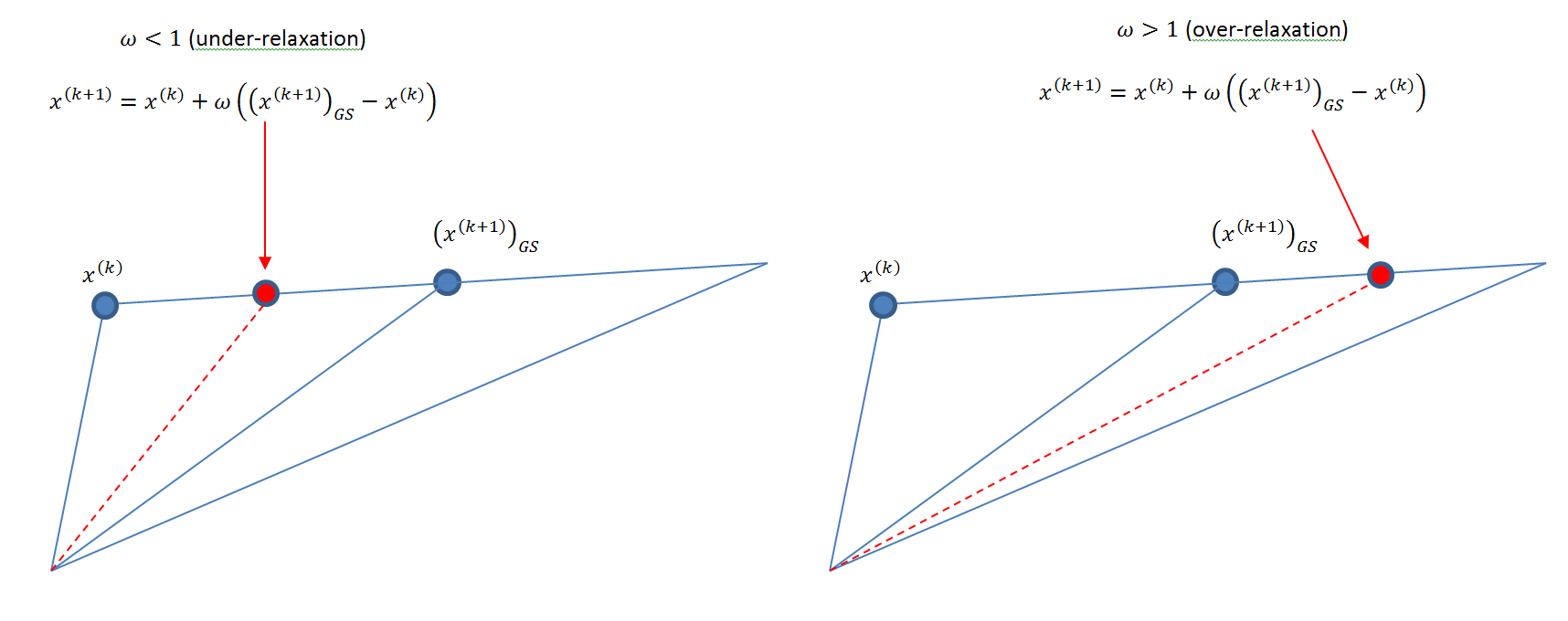
Figure 1. Illustration of under- and over-relaxation methods
Lecture Video
The following video covers the SOR method.