
Errors: Description and Definitions
Accuracy and Precision
Accuracy is the measure of how closely a computed or measured value agrees with the true value. Precision is the measure of how closely individual computed or measured values agree with each other. Figure 1 illustrates the classical example of four different situations of five dart board throws to differentiate between accuracy and precision. In the first situation, the five throws are centered around the Bull’s eye (accurate) and are close to each other (precise). In the second situation, the five throws are centered far from the Bull’s eye (inaccurate) but are close to each other (precise). In the third situation, the five throws are centered around the Bull’s eye (accurate) but are far from each other (imprecise). In the last situation, the five throws are centered far from the Bull’s eye (inaccurate) and they are far from each other (imprecise). In general, if we take the average position of the five throws, then, the distance between the average position and the Bull’s eye position would give a measure of the accuracy. On the other hand, the standard deviation of the position of the five throws gives a measure of how precise (close to each other) the throws are.
Degree of Precision
For measurement or computational systems, the degree of precision defines the smallest value that can be measured or computed. For example, the smallest division on a scientific measurement device would give the degree of precision of that device. The smallest or largest number that a computer can store defines the degree of precision of a computation by that computer.
For example, Figure 2 shows a ruler with a 1mm degree of precision. To properly record the measurement, the degree of precision has to be indicated. The measurement on the left should be recorded as  . The measurement on the right should be recorded as
  .
.
The degree of precision of a computational device depends on the algorithm of computation and storage capacity of the device. For example, a calculator might do calculations up to a particular accuracy, say ten decimal digits. Traditionally computer coding had different degrees of numerical precision for example: Single precision and double precision. The storage of numbers in these cases uses the “floating point” storage in which a number is stored as a significand and an exponent. More recently, some coding software adopt an arbitrary precision where the number of digits of precision of a number is limited only by the available memory of the computer system. It should be noted that modern computers have the ability to store enough numbers to ensure very high degree of precision for the majority of practical applications, in particular those applications described in these pages.
For the pages here we will be using Mathematica software which uses its own definitions of precision and accuracy. Numerical precision in Mathematica is defined as the number of significant decimal digits while accuracy is defined as the number of significant decimal digits to the right of the decimal point. See the Mathematica page on numerical precision for more details. As an example, consider the number  . When
  is assigned this number, it automatically adopts its precision which is 23 (23 significant digits). We can then use the command
  to set
 ![b=N[a]](https://engcourses-uofa.ca/wp-content/ql-cache/quicklatex.com-98d03e376f2d5497de25f2d0d4f68598_l3.png "Rendered by QuickLaTeX.com") . This command stores a rounded value of with machine precision (16 significant digits) into b. Therefore,
. This command stores a rounded value of with machine precision (16 significant digits) into b. Therefore,  . If we subtract
  , Mathematica uses the least precision in the calculations (machine precision) and so the result is zero. We can reset the precision of
  to be 23 significant digits. Then, in that case
  . Then, when we subtract
  we get -0.1234567.
a = 1234567890123456.1234567
b = N[a]
Precision[a]
Precision[b]
b = SetPrecision[b, 23]
b - a
import sympy as sp
import numpy as np
a = 1234567890123456.1234567
print("a:",a)
print("N(a):",sp.N(a))
toFloat32 = np.float32(a)
print("float32:",toFloat32)
toFloat64 = np.float64(toFloat32)
print("float64:",toFloat64)
print("toFloat64-a:",toFloat64-a)
Random and Systematic Errors
Using the same classical example, we can also differentiate the errors in hitting the target (i.e., the difference between the positions of the dart throws and the Bull’s eye) into two types of error: random error and systematic error. A random error is the error due to natural fluctuations in measurement or computational systems. By definition, these fluctuations are random and therefore, the average random error is zero. For the accurate throws shown in Figure 1 (left column), whether the measurements are precise or not, the average position of the five throws is the Bull’s eye. In other words, the average error is zero.
A systematic error is a repeated “bias” in the measurement or computational system. For the inaccurate throws shown in Figure 1 (right column), the thrower has a tendency or bias to throw into the left bottom side of the Bull’s eye. So, in addition to the random error, there is a systematic error (bias).
An example of a systematic error is if a scale reads 1kg when there is nothing on it so it adds 1 kg to its actual measurement. This additional 1kg is a systematic error.
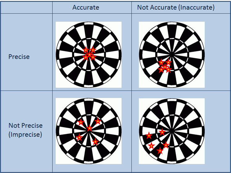
Figure 1. Illustration of accuracy and precision
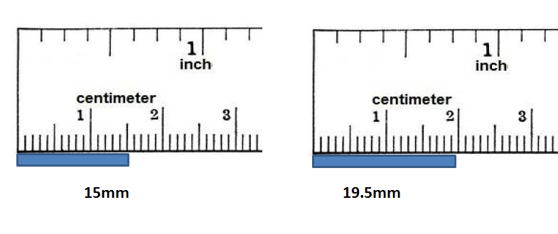
Figure 2. Degree of precision of a ruler
Basic Definitions of Errors
Measurement devices are used to find a measurement  as close as possible to the true value
  . Similarly, numerical methods often seek to find an approximation for the true solution of a problem. The error
  in a measurement or in a solution of a problem is defined as the difference between the true value and the approximation .
![\[ E=V_t-V_a \]](https://engcourses-uofa.ca/wp-content/ql-cache/quicklatex.com-7a27d5a2df96de8bd74efbb0fe278ab5_l3.png "Rendered by QuickLaTeX.com")
Another measure is the relative error  . The relative error is defined as the value of the error normalized to the true value:
![\[ E_r=\frac{E}{V_t} \]](https://engcourses-uofa.ca/wp-content/ql-cache/quicklatex.com-90ce5e5df06468ef6628239d5e039345_l3.png "Rendered by QuickLaTeX.com")
In general, if we don’t know the true value , there are methods for estimating an approximation for the error. If  is an approximation for the error, then, the relative approximate error
  is defined as:
![\[ \varepsilon_r=\frac{\varepsilon}{V_a} \]](https://engcourses-uofa.ca/wp-content/ql-cache/quicklatex.com-7461fc345f227390e34b585b47210de4_l3.png "Rendered by QuickLaTeX.com")
Word of Caution
It is important to note that for a particular computation, if the true value is equal to zero, then the relative measures of error need to be viewed carefully. In particular, in a numerical procedure, when the true value is not known, the relative error is a quantity that is approaching  which might not show any sign of convergence. In these situations, it is advisable to have other measures of convergence such as the value of the difference of the estimates or the value of itself.
Errors in Computations
There are two types of errors that arise in computations: round-off errors and truncation errors.
Round-off Errors
Round-off error is the difference between the rounding approximation of a number and its exact value. For example, in order to use the irrational number  in a computation, an approximate value is used. The difference between and the approximation represents the rounding error. For example, using 3.14 as an approximation for has a rounding approximate error of around
![\[\varepsilon_r= \frac{0.00159}{3.14}=0.0005 \]](https://engcourses-uofa.ca/wp-content/ql-cache/quicklatex.com-c28b4c140f1942abfda96919720ec5ff_l3.png "Rendered by QuickLaTeX.com")
When we use a computational device, numbers are represented in a decimal system. The precision of the computation can be defined using different ways. One way is to define the precision up to a specified decimal place. For example, the irrational number approximated to the nearest 5 decimal places is 3.14159. In this case, we know that the error is less than 0.00001. Another way is to define the precision up to a specified number of significant digits. For example, the irrational number approximated to 5 significant digits is 3.1416. Similarly, we know that the error in that case is less than 0.0001.
Round-off errors have an effect when a computation is done in multiple steps where a user is rounding off the values rather than using all the digits stored in the computer. For example, if you divide 1 by 3 in a computer, you get 0.333333333333. If you then round it to the nearest 2 decimal places, you get the number 0.33. If afterwards, you multiply 0.33 by 3, you get the value 0.99 which should have been 1 if rounding had not been used.
Even when computers are used, in very rare situations, round-off errors could lead to accumulation of errors. For example, rounding errors would be significant if we try to divide a very large number by a very small number or the other way around. Another example is if a calculation involves numerous steps and rounding is performed after every step. In these situations, the precision and/or rounding by the software or code used should be carefully examined. Some famous examples of round-off errors leading to disasters can be found here. See example 4 below for an illustration of the effect of round-off errors.
Truncation Errors
Truncation errors are errors arising when truncating an infinite sum and approximating it by a finite sum. Truncation errors arise naturally when using the Taylor series, numerical integration, and numerical differentiation. These will be covered later along with their associated truncation errors. For example, as will be shown later, the  function can be represented using the infinite sum:
![\[ \sin(x)=x-\frac{x^3}{3!}+\frac{x^5}{5!}-\frac{x^7}{7!}+\cdots = \sum_{n=0}^\infty\frac{(-1)^n}{(2n+1)!}x^{2n+1} \]](https://engcourses-uofa.ca/wp-content/ql-cache/quicklatex.com-6160a23facca9ef942ff22361b2a8a2f_l3.png "Rendered by QuickLaTeX.com")
In fact, this is how a calculator calculates the sine of an angle. Using the above series,  where 0.3 is in radian can be calculated using the first two terms as:
![\[ \sin(0.3)=0.3-\frac{0.3^3}{3\times 2}=0.2955 \]](https://engcourses-uofa.ca/wp-content/ql-cache/quicklatex.com-55ff5915c51f3ea2f8a89d127105a090_l3.png "Rendered by QuickLaTeX.com")
which in fact is a very good approximation to the actual value which is around 0.295520207. The error, or the difference between 0.2955 and 0.295520207 is called a truncation error arising from using a finite number of terms (in this case only 2) in the infinite series.
Error Estimation in Computational Iterative Methods
If the approximate value is obtained using an iterative method, i.e., each iteration  would produce the approximation
  , then, the relative approximate error is defined as:
![\[ \varepsilon_r=\frac{{V_a}_n-{V_a}_{n-1}}{{V_a}_n} \]](https://engcourses-uofa.ca/wp-content/ql-cache/quicklatex.com-b764617c10d3e19df52dac433e2f18a3_l3.png "Rendered by QuickLaTeX.com")
In such cases, the iterative method can be stopped when the absolute value of the relative error reaches a specified error level  :
:
![\[ |\varepsilon_r|\leq \varepsilon_s \]](https://engcourses-uofa.ca/wp-content/ql-cache/quicklatex.com-74ff9283a69af7722ff6bee2a241846e_l3.png "Rendered by QuickLaTeX.com")