
Numerical Differentiation: Effect of Data Errors
Effect of Data Errors
One of the major problems when numerically differentiating empirical data is the existence of random (measurement) errors within the data itself. These errors cause the experimental data to have some natural fluctuations. If the experimental data is supposed to follow a particular model, then the best way to deal with such data is to find the best fit and use the derivatives of the best fit as described in the curve fitting section. However, if such a model does not exist, for example when measuring the position function of a moving subject, then care has to be taken when dealing with higher derivatives of the data. In particular, the fluctuations are magnified when higher derivatives are calculated.
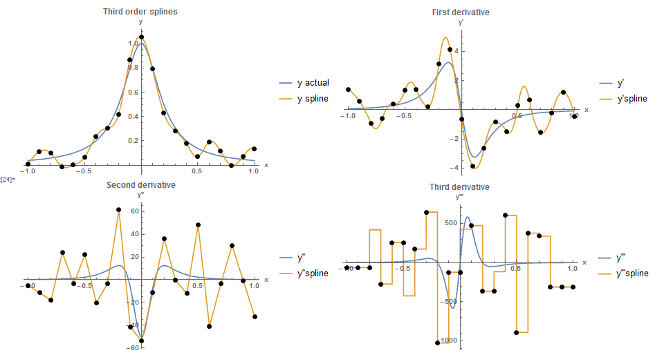
The following figures were generated by first sampling the Runge function on the domain ![[-1,1]](https://engcourses-uofa.ca/wp-content/ql-cache/quicklatex.com-4a7430a5619e08a23c430423c1376967_l3.png "Rendered by QuickLaTeX.com") at an interval of
at an interval of  , then a random number between -0.1 and 0.1 is added to the data points. A cubic spline is then fit into the data. The small fluctuations in the data lead to very high fluctuations in all the derivatives. In particular, the second and third derivatives do not provide any useful information.
Clear[x]
h = 0.1;
n = 2/h + 1;
y = 1/(1 + 25 x^2);
yp = D[y, x];
ypp = D[yp, x];
yppp = D[ypp, x];
ypppp = D[yppp, x];
Data = Table[{-1 + h*(i - 1), (y /. x -> -1 + h*(i - 1)) +RandomReal[{-0.1, 0.1}]}, {i, 1, n}];
y2 = Interpolation[Data, Method -> "Spline", InterpolationOrder -> 3];
ypInter = D[y2[x], x];
yppInter = D[y2[x], {x, 2}];
ypppInter = D[y2[x], {x, 3}];
yppppInter = D[y2[x], {x, 4}];
Data1 = Table[{Data[[i, 1]], (ypInter /. x -> Data[[i, 1]])}, {i, 1, n}];
Data2 = Table[{Data[[i, 1]], (yppInter /. x -> Data[[i, 1]])}, {i, 1,n}];
Data3 = Table[{Data[[i, 1]], (ypppInter /. x -> Data[[i, 1]])}, {i, 1, n}];
Data4 = Table[{Data[[i, 1]], (yppppInter /. x -> Data[[i, 1]])}, {i, 1, n}];
a0 = Plot[{y, y2[x]}, {x, -1, 1}, Epilog -> {PointSize[Large], Point[Data]}, AxesLabel -> {"x", "y"}, BaseStyle -> Bold, ImageSize -> Medium, PlotRange -> All, PlotLegends -> {"y actual", "y spline"},  PlotLabel -> "Third order splines"];
a1 = Plot[{yp, ypInter}, {x, -1, 1}, Epilog -> {PointSize[Large], Point[Data1]}, AxesLabel -> {"x", "y'"}, BaseStyle -> Bold, ImageSize -> Medium, PlotRange -> All, PlotLegends -> {"y'", "y'spline"},  PlotLabel -> "First derivative"];
a2 = Plot[{ypp, yppInter}, {x, -1, 1}, Epilog -> {PointSize[Large], Point[Data2]}, AxesLabel -> {"x", "y''"}, BaseStyle -> Bold, ImageSize -> Medium,  PlotRange -> All, PlotLegends -> {"y''", "y''spline"},   PlotLabel -> "Second derivative"];
a3 = Plot[{yppp, ypppInter}, {x, -1, 1},    Epilog -> {PointSize[Large], Point[Data3]},    AxesLabel -> {"x", "y'''"}, BaseStyle -> Bold, ImageSize -> Medium,    PlotRange -> All, PlotLegends -> {"y'''", "y'''spline"},    PlotLabel -> "Third derivative"];
a4 = Plot[{ypppp, yppppInter}, {x, -1, 1},    Epilog -> {PointSize[Large], Point[Data4]},    AxesLabel -> {"x", "y''''"}, BaseStyle -> Bold, ImageSize -> Medium,    PlotRange -> All, PlotLegends -> {"y''''", "y''''spline"},    PlotLabel -> "Fourth derivative"];
Grid[{{a0,a1}, {a2,a3}}]
import random
import numpy as np
import sympy as sp
import matplotlib.pyplot as plt
from scipy.interpolate import UnivariateSpline

x = sp.symbols('x')
x_val = np.arange(-1, 1,0.01)
h = 0.1
n = int(2/h + 1)
y = 1/(1 + 25*x**2)
yp = y.diff(x, n=1)
ypp = yp.diff(x, n=2)
yppp = ypp.diff(x, n=3)
Data = [[-1 + h*i, (y.subs(x, -1 + h*i)) + random.uniform(-0.1, 0.1)] for i in range(n)]

y2 = UnivariateSpline([point[0] for point in Data],[point[1] for point in Data], k=3, s=0)
ypInter = y2.derivative(1)
yppInter = y2.derivative(2)
ypppInter = y2.derivative(3)

Data1 = [[point[0], ypInter(point[0])] for point in Data]
Data2 = [[point[0], yppInter(point[0])] for point in Data]
Data3 = [[point[0], ypppInter(point[0])] for point in Data]

plt.title("Third order splines")
plt.xlabel("x"); plt.ylabel("y")
plt.scatter([point[0] for point in Data],[point[1] for point in Data], c='k')
plt.plot(x_val, [y.subs(x,i) for i in x_val], label="y actual")
plt.plot(x_val, [y2(i) for i in x_val], label="y spline")
plt.legend(); plt.grid(); plt.show()

plt.title("First derivative")
plt.xlabel("x"); plt.ylabel("y'")
plt.scatter([point[0] for point in Data1],[point[1] for point in Data1], c='k')
plt.plot(x_val, [yp.subs(x,i) for i in x_val], label="y'")
plt.plot(x_val, [ypInter(i) for i in x_val], label="y'spline")
plt.legend(); plt.grid(); plt.show()

plt.title("Second derivative")
plt.xlabel("x"); plt.ylabel("y''")
plt.scatter([point[0] for point in Data2],[point[1] for point in Data2], c='k')
plt.plot(x_val, [ypp.subs(x,i) for i in x_val], label="y''")
plt.plot(x_val, [yppInter(i) for i in x_val], label="y''spline")
plt.legend(); plt.grid(); plt.show()

plt.title("Third derivative")
plt.xlabel("x"); plt.ylabel("y'''")
plt.scatter([point[0] for point in Data3],[point[1] for point in Data3], c='k')
plt.plot(x_val, [yppp.subs(x,i) for i in x_val], label="y'''")
plt.plot(x_val, [ypppInter(i) for i in x_val], label="y'''spline")
plt.legend(); plt.grid(); plt.show()
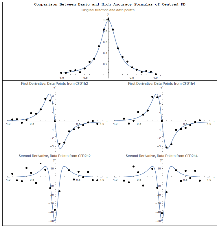
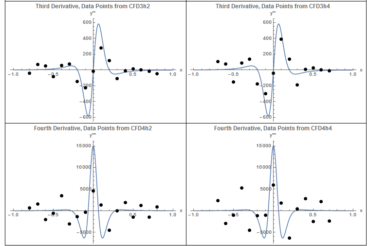
Similarly, the shown figures show the results when random numbers between -0.05 and 0.05 are added to the sampled data of the Runge function. When the centred finite difference scheme is used, the errors lead to very large variations in the second and third derivatives. The fourth derivative does not provide any useful information.
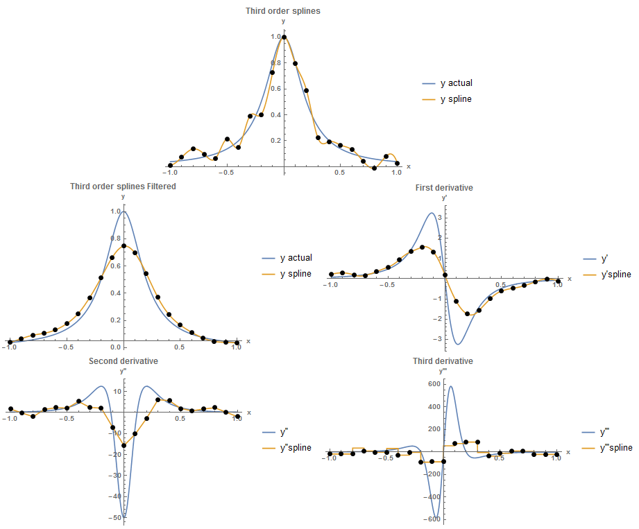
One possible solution to reduce noise in the data is to use a “Filter” to smooth the data. In the following figure, the built-in Gaussian Filter in Mathematica is used to reduce the generated noise. The fluctuations in the data are reduced and smoother derivatives are obtained.
Clear[x]
h = 0.1;
n = 2/h + 1;
y = 1/(1 + 25 x^2);
yp = D[y, x];
ypp = D[yp, x];
yppp = D[ypp, x];
ypppp = D[yppp, x];
Data = Table[{-1 + h*(i - 1), (y /. x -> -1 + h*(i - 1)) +    RandomReal[{-0.1, 0.1}]}, {i, 1, n}];
Dataa = Data;
f = Data[[All, 2]];
f = GaussianFilter[f, 3];
Data = Table[{Data[[i, 1]], f[[i]]}, {i, 1, n}];
yun = Interpolation[Dataa, Method -> "Spline",   InterpolationOrder -> 3];
y2 = Interpolation[Data, Method -> "Spline", InterpolationOrder -> 3];
ypInter = D[y2[x], x];
yppInter = D[y2[x], {x, 2}];
ypppInter = D[y2[x], {x, 3}];
yppppInter = D[y2[x], {x, 4}];
Data1 = Table[{Data[[i, 1]], (ypInter /. x -> Data[[i, 1]])}, {i, 1,  n}];
Data2 = Table[{Data[[i, 1]], (yppInter /. x -> Data[[i, 1]])}, {i, 1, n}];
Data3 = Table[{Data[[i, 1]], (ypppInter /. x -> Data[[i, 1]])}, {i, 1, n}];
Data4 = Table[{Data[[i, 1]], (yppppInter /. x -> Data[[i, 1]])}, {i, 1, n}];
aun = Plot[{y, yun[x]}, {x, -1, 1}, Epilog -> {PointSize[Large], Point[Dataa]}, AxesLabel -> {"x", "y"}, BaseStyle -> Bold, ImageSize -> Medium, PlotRange -> All, PlotLegends -> {"y actual", "y spline"}, PlotLabel -> "Third order splines"];
a0 = Plot[{y, y2[x]}, {x, -1, 1},    Epilog -> {PointSize[Large], Point[Data]}, AxesLabel -> {"x", "y"},    BaseStyle -> Bold, ImageSize -> Medium, PlotRange -> All,    PlotLegends -> {"y actual", "y spline"},    PlotLabel -> "Third order splines Filtered"];
a1 = Plot[{yp, ypInter}, {x, -1, 1},    Epilog -> {PointSize[Large], Point[Data1]},    AxesLabel -> {"x", "y'"}, BaseStyle -> Bold, ImageSize -> Medium,    PlotRange -> All, PlotLegends -> {"y'", "y'spline"},    PlotLabel -> "First derivative"];
a2 = Plot[{ypp, yppInter}, {x, -1, 1},    Epilog -> {PointSize[Large], Point[Data2]},    AxesLabel -> {"x", "y''"}, BaseStyle -> Bold, ImageSize -> Medium,    PlotRange -> All, PlotLegends -> {"y''", "y''spline"},    PlotLabel -> "Second derivative"];
a3 = Plot[{yppp, ypppInter}, {x, -1, 1},    Epilog -> {PointSize[Large], Point[Data3]},    AxesLabel -> {"x", "y'''"}, BaseStyle -> Bold, ImageSize -> Medium,    PlotRange -> All, PlotLegends -> {"y'''", "y'''spline"},    PlotLabel -> "Third derivative"];
a4 = Plot[{ypppp, yppppInter}, {x, -1, 1},    Epilog -> {PointSize[Large], Point[Data4]},    AxesLabel -> {"x", "y''''"}, BaseStyle -> Bold, ImageSize -> Medium,    PlotRange -> All, PlotLegends -> {"y''''", "y''''spline"},    PlotLabel -> "Fourth derivative"];
Grid[{{aun, SpanFromLeft}, {a0, a1}, {a2, a3}}]
import random
import sympy as sp
import numpy as np
import matplotlib.pyplot as plt
from scipy.ndimage import gaussian_filter
from scipy.interpolate import UnivariateSpline

x = sp.symbols('x')
x_val = np.arange(-1, 1,0.01)
h = 0.1
n = int(2/h + 1)
y = 1/(1 + 25*x**2)
yp = sp.diff(y, x, n=1)
ypp = sp.diff(yp, x, n=2)
yppp = sp.diff(ypp, x, n=3)
Data = np.array([[-1 + h*i, (y.subs(x, -1 + h*i)) + random.uniform(-0.1, 0.1)] for i in range(n)])
Dataa = Data.copy()
f = Data[:, 1]
f = gaussian_filter(np.float_(f), sigma=1)
Data = [[Data[i][0], f[i]] for i in range(n)]

yun = UnivariateSpline([point[0] for point in Dataa],[point[1] for point in Dataa], k=3, s=0)
y2 = UnivariateSpline([point[0] for point in Data],[point[1] for point in Data], k=3, s=0)
ypInter = y2.derivative(1)
yppInter = y2.derivative(2)
ypppInter = y2.derivative(3)

Data1 = [[point[0], ypInter(point[0])] for point in Data]
Data2 = [[point[0], yppInter(point[0])] for point in Data]
Data3 = [[point[0], ypppInter(point[0])] for point in Data]

plt.title("Third order splines")
plt.xlabel("x"); plt.ylabel("y")
plt.scatter([point[0] for point in Dataa],[point[1] for point in Dataa], c='k')
plt.plot(x_val, [y.subs(x,i) for i in x_val], label="y actual")
plt.plot(x_val, [yun(i) for i in x_val], label="y spline")
plt.legend(); plt.grid(); plt.show()

plt.title("Third order splines Filtered")
plt.xlabel("x"); plt.ylabel("y")
plt.scatter([point[0] for point in Data],[point[1] for point in Data], c='k')
plt.plot(x_val, [y.subs(x,i) for i in x_val], label="y actual")
plt.plot(x_val, [y2(i) for i in x_val], label="y spline")
plt.legend(); plt.grid(); plt.show()

plt.title("First derivative")
plt.xlabel("x"); plt.ylabel("y'")
plt.scatter([point[0] for point in Data1],[point[1] for point in Data1], c='k')
plt.plot(x_val, [yp.subs(x,i) for i in x_val], label="y'")
plt.plot(x_val, [ypInter(i) for i in x_val], label="y'spline")
plt.legend(); plt.grid(); plt.show()

plt.title("Second derivative")
plt.xlabel("x"); plt.ylabel("y''")
plt.scatter([point[0] for point in Data2],[point[1] for point in Data2], c='k')
plt.plot(x_val, [ypp.subs(x,i) for i in x_val], label="y''")
plt.plot(x_val, [yppInter(i) for i in x_val], label="y''spline")
plt.legend(); plt.grid(); plt.show()

plt.title("Third derivative")
plt.xlabel("x"); plt.ylabel("y'''")
plt.scatter([point[0] for point in Data3],[point[1] for point in Data3], c='k')
plt.plot(x_val, [yppp.subs(x,i) for i in x_val], label="y'''")
plt.plot(x_val, [ypppInter(i) for i in x_val], label="y'''spline")
plt.legend(); plt.grid(); plt.show()